03 Testing Fundamentals: Unit Testing - Equivalence Classes
April 2026 (17818 Words, 99 Minutes)
Chapter 03: Unit Testing - Equivalence Classes
Prerequisites: This lecture continues from Chapter 03 (Testing Basics): Testing Fundamentals - Basics. Make sure you understand the testing pyramid, AAA pattern, and clean code principles before proceeding.
1. Introduction: The Test Selection Problem
In Part 1, we learned:
- How to write unit tests using pytest
- The AAA pattern (Arrange-Act-Assert)
- Clean code principles for tests
But we glossed over a crucial question: Which tests should you write?
Consider a simple function:
def reciprocal(x: float) -> float:
    return 1.0 / x
There are infinitely many possible inputs. You can’t test them all. How do you choose?
This lecture answers that question using equivalence class partitioning - a systematic approach to selecting test cases that maximize coverage while minimizing redundancy.
1.1 Equivalence Classes: Finding Them is Hard
We’ve established that exhaustive testing is impossible (Section 5.3), so we need a smarter strategy. That strategy is equivalence class partitioning - grouping similar inputs and testing representatives from each group. This works well for simple cases, but finding equivalence classes gets dramatically harder as functions become more complex.
What is an Equivalence Class? (Accessible Definition)
Equivalence Class: A set of inputs that are expected to be processed in the same way by the function under test, producing the same category of output or behavior.
In plain language:
- An equivalence class groups inputs that should behave similarly
- All inputs within one subset should trigger the same code paths and produce similar behavior
- If one input in a class passes its test, we assume all inputs in that class would also pass
- If one fails, we assume the entire class has a problem
Key properties:
- Disjoint: No input belongs to multiple classes
- Complete: Every possible input belongs to exactly one class
- Representative testing: Test one value from each class (not all values)
The Mathematical Foundation (For the Curious)
For those comfortable with mathematics, here’s the precise definition that explains why equivalence classes work:
Given:
- A function \(f: D\subset \mathbb{R} \rightarrow \mathbb{R}\) (Domain → Range)
- A partition of the output range into output categories \(C_1, C_2, \ldots, C_n\)
Define an equivalence relation on inputs:
\[x \sim y \iff f(x) \text{ and } f(y) \text{ belong to the same output category } C_i\]This means: “Two inputs \(x\) and \(y\) are equivalent if their outputs fall in the same category.”
Then the equivalence classes are:
\[E_i = \{ x \in D : f(x) \in C_i \}\]Each equivalence class \(E_i\) is the set of all inputs that map to output category \(C_i\).
Critical insight: The number of equivalence classes equals the number of output categories you define!
- Choose 3 output categories → get 3 equivalence classes
- Choose 4 output categories → get 4 equivalence classes
- The partition is a choice based on what matters for testing
Example with reciprocal(x) = 1/x:
If we partition the output range as: \(\{\text{positive}, \text{negative}, \text{error}\}\)
Then the input equivalence classes are:
- \(E_1 = \{x : x > 0\}\) (inputs producing positive outputs)
- \(E_2 = \{x : x < 0\}\) (inputs producing negative outputs)
- \(E_3 = \{x : x = 0\}\) (inputs producing errors)
Notice: \(E_1 \cup E_2 \cup E_3 = \mathbb{R}\) (all real numbers) - the union covers the entire input domain!
1.1.1 Generalization to Multiple Dimensions
The definition above works for any input and output dimensions:
For a function \(f: \mathbb{R}^n \rightarrow \mathbb{R}^m\) (n inputs, m outputs):
- Partition the m-dimensional output space \(\mathbb{R}^m\) into categories \(C_1, C_2, \ldots, C_k\)
- Each \(C_i \subseteq \mathbb{R}^m\) is a subset of the output space
-
The equivalence classes partition the n-dimensional input space \(\mathbb{R}^n\):
\[E_i = \{ (x_1, x_2, \ldots, x_n) \in \mathbb{R}^n : f(x_1, \ldots, x_n) \in C_i \}\] -
The union covers the entire input domain:
\[E_1 \cup E_2 \cup \cdots \cup E_k = \mathbb{R}^n\]
Examples from this lecture:
| Function | Input Space | Output Space | Partitioning |
|---|---|---|---|
reciprocal(x) |
\(\mathbb{R}\) (1D) | \(\mathbb{R} \cup \{\text{error}\}\) (1D + error) | 3 output categories → 3 input classes |
reciprocal_sum(x,y,z) |
\(\mathbb{R}^3\) (3D) | \(\mathbb{R} \cup \{\text{error}\}\) (1D + error) | 3 output categories → 3 input classes |
calculate_ray_slope(angle) |
\(\mathbb{R}\) (1D) | \(\mathbb{R} \cup \{\text{None}\}\) (1D + special) | 4 output categories → 4 input classes |
find_intersection(...) |
\(\mathbb{R}^n \times \mathbb{R} \times \mathbb{R} \times \mathbb{R}\) | \(\mathbb{R}^3 \cup \{(None, None, None)\}\) | Many categories → many classes |
Key insight: Regardless of dimensions:
- You partition the output space (whatever dimension it is)
- This induces a partition on the input space (whatever dimension it is)
- The number of input equivalence classes equals the number of output categories you define
Why this matters:
reciprocal_sum(x,y,z)takes 3 inputs but still has only 3 equivalence classes (not 3³ = 27!)- The output is 1-dimensional (just a float), partitioned into {positive, negative, error}
- All input triples
(x,y,z)that produce positive output form ONE equivalence class, regardless of individual signs
1.1.2 How Do I Choose the Output Categories \(C_1, C_2, \ldots, C_n\)? Is This Unique?
Short answer: No, the choice is NOT unique! You choose based on what matters for your testing goals.
The mathematical definition tells us:
- Partition the output space into categories \(C_1, C_2, \ldots, C_n\)
- This induces the input equivalence classes \(E_1, E_2, \ldots, E_n\)
But it doesn’t tell us HOW to partition! This is a design choice based on:
1. What behaviors do you care about?
For reciprocal(x) = 1/x, you could choose:
Coarse partition (2 output categories):
- \(C_1 = \{\text{valid output}\}\) (any real number)
- \(C_2 = \{\text{error}\}\)
This gives 2 input equivalence classes:
- \(E_1 = \{x : x \neq 0\}\) (all non-zero inputs)
- \(E_2 = \{x : x = 0\}\) (zero)
Fine partition (3 output categories - what we chose):
- \(C_1 = \{y : y > 0\}\) (positive outputs)
- \(C_2 = \{y : y < 0\}\) (negative outputs)
- \(C_3 = \{\text{error}\}\)
This gives 3 input equivalence classes:
- \(E_1 = \{x : x > 0\}\) (positive inputs)
- \(E_2 = \{x : x < 0\}\) (negative inputs)
- \(E_3 = \{x : x = 0\}\) (zero)
Very fine partition (5 output categories - overkill):
- \(C_1 = \{y : y > 1\}\) (output greater than 1)
- \(C_2 = \{y : 0 < y \leq 1\}\) (output between 0 and 1)
- \(C_3 = \{y : -1 \leq y < 0\}\) (output between -1 and 0)
- \(C_4 = \{y : y < -1\}\) (output less than -1)
- \(C_5 = \{\text{error}\}\)
This gives 5 input equivalence classes:
- \(E_1 = \{x : 0 < x < 1\}\) (inputs between 0 and 1)
- \(E_2 = \{x : x \geq 1\}\) (inputs ≥ 1)
- \(E_3 = \{x : -1 \leq x < 0\}\) (inputs between -1 and 0)
- \(E_4 = \{x : x < -1\}\) (inputs < -1)
- \(E_5 = \{x : x = 0\}\) (zero)
All three are mathematically valid! But which is best for testing?
2. Trade-off: Granularity vs. Practicality
| Partition Choice | # Tests | Pros | Cons |
|---|---|---|---|
| Coarse (2) | 2 tests | Fast, minimal | Might miss sign-related bugs |
| Fine (3) | 3 tests | Good balance, catches sign bugs | Still practical |
| Very fine (5) | 5 tests | Maximum coverage | Overkill for simple function, diminishing returns |
We chose the fine partition (3 categories) because:
- ✅ Separating positive/negative catches sign bugs (common in math functions)
- ✅ Only requires 3 tests (practical)
- ✅ Aligns with typical behavior categories for reciprocal functions
- ❌ The coarse partition (2 categories) misses potential sign bugs
- ❌ The very fine partition (5 categories) adds tests without much extra value
3. Guidelines for Choosing Output Categories
Choose your partition based on:
| Consideration | Question to Ask | Example |
|---|---|---|
| Code paths | Does the code branch based on this output category? | If if result > 0: ... exists, positive/negative matter |
| Mathematical properties | Does this output value have special significance? | Zero, infinity, special constants |
| Domain significance | Do different output ranges mean different things to users? | In ray tracing, None vs. coordinates are fundamentally different |
| Bug risk | Where are bugs most likely? | Sign errors are common → separate positive/negative |
| Practical limit | How many tests can you maintain? | 3-5 classes per dimension is usually enough |
4. The Key Insight: You Control the Granularity
The mathematical definition does not mandate a specific partition. It only requires:
\[C_1 \cup C_2 \cup \cdots \cup C_n = \text{(entire output range)}\] \[C_i \cap C_j = \emptyset \quad \text{for } i \neq j\]You choose how to slice the output space. Different slicing → different equivalence classes → different tests.
Bottom line: Start with 3-4 output categories based on code behavior and mathematical significance. Refine if you find bugs that weren’t caught.
1.1.3 White-Box vs. Black-Box: How Do We Know Where to Partition?
Important clarification: The approach we’re using here is white-box testing - we can see the implementation.
Why does this matter?
Consider reciprocal_sum(x, y, z). How do we know to partition based on \(x+y+z\)?
Because we can see the code:
def reciprocal_sum(x: float, y: float, z: float) -> float:
    total = x + y + z  # ← THIS tells us to partition on the sum!
    if abs(total) < 1e-10:
        raise ZeroDivisionError("Sum is too close to zero")
    return 1.0 / total
The implementation reveals:
- The function computes
x + y + z(so the sum matters, not individual values) - It returns
1/total(so sign of total matters: positive/negative) - It checks
abs(total) < 1e-10(so near-zero is special)
This immediately tells us the 3 output categories: positive, negative, error.
Without seeing the code (black-box testing):
If we only had the function signature:
def reciprocal_sum(x: float, y: float, z: float) -> float:
    """Return the reciprocal of the sum of x, y, and z."""
We’d need to guess partitions based on:
- Function name: “reciprocal_sum” suggests it sums first
- Docstring: confirms it’s
1/(x+y+z) - Mathematical reasoning: reciprocal fails at zero
But white-box is easier and more accurate - you see exactly what the code does!
For this lecture: All examples are white-box - we look at the code to find partitions. This is:
- ✅ Practical: You write the code, you see the implementation
- ✅ Accurate: You know exactly what branches exist
- ✅ Realistic: Most unit testing in real projects is white-box
When do you use black-box? Testing external libraries/APIs where you don’t have source code. That’s more advanced.
This section demonstrates:
- Simple functions → Easy to find equivalence classes
- Multiple parameters → Classes multiply quickly
- Array inputs → Structural AND value classes
- Complex functions → Even AI assistants struggle
Let’s build intuition with progressive examples, from trivial to realistic.
1.1.4 Simple Float Example: reciprocal(x) = 1/x
Function Definition:
def reciprocal(x: float) -> float:
    """Return the reciprocal of x (1/x)."""
    if x == 0:
        raise ZeroDivisionError("Cannot divide by zero")
    return 1.0 / x
Question: What are the equivalence classes for parameter x?
Intuitive Approach (White-Box Testing):
Since we can see the implementation, let’s identify special cases naturally:
Looking at the code, we immediately notice:
-
x = 0is special - The code explicitly checks for it withif x == 0and raises an error. This is clearly a different behavior category! - Positive vs. Negative matters - For the reciprocal function
1/x:- When
x > 0(likex = 5.0), we get a positive result (1/5 = 0.2) - When
x < 0(likex = -5.0), we get a negative result (1/(-5) = -0.2) - The sign of the input determines the sign of the output!
- When
- These are distinct behaviors - The function behaves fundamentally differently for positive, negative, and zero inputs.
So we naturally identify 3 equivalence classes:
| Equivalence Class | Description | Representative Value | Expected Behavior |
|---|---|---|---|
| Positive numbers | x > 0 |
x = 5.0 |
Returns positive reciprocal (0.2) |
| Negative numbers | x < 0 |
x = -5.0 |
Returns negative reciprocal (-0.2) |
| Zero | x == 0 |
x = 0.0 |
Raises ZeroDivisionError |
Why these three classes?
This partitioning comes directly from understanding the code:
- Zero is special - It triggers the error-handling branch (
if x == 0) - Sign matters - Positive and negative inputs follow the same code path (
return 1.0 / x) but produce outputs with different signs - All inputs are covered - Every possible float is either positive, negative, or zero
Test Code:
import pytest

def test_reciprocal_positive_number():
    """Equivalence class: Positive numbers (x > 0)"""
    result = reciprocal(5.0)
    assert result == pytest.approx(0.2, rel=1e-10)

def test_reciprocal_negative_number():
    """Equivalence class: Negative numbers (x < 0)"""
    result = reciprocal(-5.0)
    assert result == pytest.approx(-0.2, rel=1e-10)

def test_reciprocal_zero():
    """Equivalence class: Zero (x == 0)"""
    with pytest.raises(ZeroDivisionError):
        reciprocal(0.0)
For the Curious: Mathematical Formalization
The intuitive approach above can be formalized using the mathematical definition from Section 5.7. Here’s how:
-
Define the function: \(f(x) = \frac{1}{x}\) with domain \(D = \mathbb{R}\)
- Partition the output range into categories:
- \(C_1 = \{y : y > 0\}\) (positive outputs)
- \(C_2 = \{y : y < 0\}\) (negative outputs)
- \(C_3 = \{\text{error}\}\) (division by zero)
-
The equivalence relation: Two inputs \(x_1 \sim x_2\) if \(f(x_1)\) and \(f(x_2)\) belong to the same output category \(C_i\)
- The induced input equivalence classes:
- \(E_1 = \{x \in \mathbb{R} : f(x) \in C_1\} = \{x : x > 0\}\) (positive inputs → positive outputs)
- \(E_2 = \{x \in \mathbb{R} : f(x) \in C_2\} = \{x : x < 0\}\) (negative inputs → negative outputs)
- \(E_3 = \{x \in \mathbb{R} : f(x) \in C_3\} = \{x : x = 0\}\) (zero → error)
- Verify the partition:
- \(E_1 \cup E_2 \cup E_3 = \mathbb{R}\) ✅ (covers all real numbers)
- \(E_i \cap E_j = \emptyset\) for \(i \neq j\) ✅ (no overlap)
The mathematical formalization confirms what we discovered intuitively: the output categories (\(C_1, C_2, C_3\)) directly determine the input equivalence classes (\(E_1, E_2, E_3\)).
What about near-zero and very large values?
You might wonder: “What about x = 0.001 (near zero) or x = 1e10 (very large)?”
These are still within the positive numbers equivalence class - they follow the same code path and produce the same category of behavior (positive output). However, they represent boundary values that might expose numerical precision issues or extreme behavior:
- Near zero (x = 0.001): Returns very large value (1000.0) - tests floating-point limits
- Very large (x = 1e10): Returns very small value (1e-10) - tests underflow behavior
These boundary values are important but belong to a different testing technique - we’ll cover Boundary Value Analysis in the next lecture. For now, recognize that:
- Equivalence classes partition inputs by behavior
- Boundary values test the edges of those partitions
Key Insight: Even a simple one-parameter function has 3 core equivalence classes. By testing one representative from each class, we achieve high confidence without exhaustive testing.
1.1.5 Multiple Parameters: reciprocal_sum(x, y, z) = 1/(x+y+z)
Function Definition:
def reciprocal_sum(x: float, y: float, z: float) -> float:
    """Return the reciprocal of the sum of x, y, and z."""
    total = x + y + z
    if abs(total) < 1e-10:
        raise ZeroDivisionError("Sum is too close to zero")
    return 1.0 / total
Question: What are the equivalence classes now?
Intuitive Approach (White-Box Testing):
Now we have 3 parameters! But let’s look at the code to understand what matters:
Looking at the code, we immediately notice:
-
The function computes
total = x + y + z- This tells us that what matters is the sum, not the individual values ofx,y, orz! -
Near-zero sum is special - The code checks
if abs(total) < 1e-10and raises an error. This is a special behavior category. - Sign of the sum matters - The function returns
1.0 / total:- When
total > 0(like1.0 + 2.0 + 3.0 = 6.0), we get a positive result (1/6 ≈ 0.167) - When
total < 0(like-1.0 + (-2.0) + (-3.0) = -6.0), we get a negative result (-1/6 ≈ -0.167)
- When
- Individual parameter signs don’t matter - As long as the sum is the same!
(1.0, 2.0, 3.0)→ sum = 6 → positive output(100.0, -50.0, -44.0)→ sum = 6 → same positive output- Both are in the same equivalence class because they have the same sum!
So we naturally identify 3 equivalence classes (same as before!):
| Equivalence Class | Description | Representative Values | Expected Behavior |
|---|---|---|---|
| Positive sum | x+y+z > 0 |
(1.0, 2.0, 3.0) → sum=6 |
Returns positive reciprocal (≈0.167) |
| Negative sum | x+y+z < 0 |
(-1.0, -2.0, -3.0) → sum=-6 |
Returns negative reciprocal (≈-0.167) |
| Zero sum | |x+y+z| < 1e-10 |
(1.0, -0.5, -0.5) → sum≈0 |
Raises ZeroDivisionError |
Key insight: Even though we have 3 input parameters, we still only have 3 equivalence classes! Why? Because the function’s behavior depends only on the sum, not on individual parameter values.
Why these three classes?
This partitioning comes directly from understanding the code:
- The sum is computed first - The line
total = x + y + ztells us that individual values don’t matter, only their sum - Zero sum is special - It triggers the error-handling branch (
if abs(total) < 1e-10) - Sign of sum matters - Positive and negative sums follow the same code path (
return 1.0 / total) but produce outputs with different signs - All input combinations are covered - Every possible triple
(x, y, z)produces a sum that is either positive, negative, or near-zero
Test Code:
import pytest

def test_reciprocal_sum_positive_total():
    """Equivalence class: Positive sum (x+y+z > 0)"""
    result = reciprocal_sum(1.0, 2.0, 3.0)  # sum = 6
    assert result == pytest.approx(1.0 / 6.0, rel=1e-10)

def test_reciprocal_sum_negative_total():
    """Equivalence class: Negative sum (x+y+z < 0)"""
    result = reciprocal_sum(-1.0, -2.0, -3.0)  # sum = -6
    assert result == pytest.approx(-1.0 / 6.0, rel=1e-10)

def test_reciprocal_sum_zero_total():
    """Equivalence class: Zero sum (x+y+z ≈ 0)"""
    with pytest.raises(ZeroDivisionError):
        reciprocal_sum(1.0, -0.5, -0.5)  # sum = 0.0
For the Curious: Mathematical Formalization
The intuitive approach above can be formalized using the mathematical definition from Section 5.7. Here’s how:
-
Define the function: \(f(x, y, z) = \frac{1}{x+y+z}\) with domain \(D = \mathbb{R}^3\) (3-dimensional input space)
- Partition the output range into categories:
- \(C_1 = \{w : w > 0\}\) (positive outputs)
- \(C_2 = \{w : w < 0\}\) (negative outputs)
- \(C_3 = \{\text{error}\}\) (sum too close to zero)
-
The equivalence relation: Two input triples \((x_1, y_1, z_1) \sim (x_2, y_2, z_2)\) if their outputs belong to the same category
- The induced input equivalence classes in \(\mathbb{R}^3\):
- \(E_1 = \{(x,y,z) \in \mathbb{R}^3 : x+y+z > 0\}\) (positive sum → positive output)
- \(E_2 = \{(x,y,z) \in \mathbb{R}^3 : x+y+z < 0\}\) (negative sum → negative output)
- \(E_3 = \{(x,y,z) \in \mathbb{R}^3 : \lvert x+y+z \rvert < 10^{-10}\}\) (near-zero sum → error)
- Verify the partition:
- \(E_1 \cup E_2 \cup E_3 = \mathbb{R}^3\) ✅ (covers all input triples)
- \(E_i \cap E_j = \emptyset\) for \(i \neq j\) ✅ (no overlap)
Important mathematical insight:
The triples (1.0, 2.0, 3.0) and (100.0, -50.0, -44.0) are in the same equivalence class \(E_1\) because:
Both satisfy \(x+y+z = 6 > 0\), so both belong to \(E_1 = \{(x,y,z) : x+y+z > 0\}\).
They produce outputs in the same category (\(C_1\) = positive), even though individual parameter values are wildly different! This is the power of the equivalence relation - it groups inputs by their behavioral outcome, not by their individual values.
What about mixed signs or near-zero sums?
You might ask: “What about inputs like (1.0, 2.0, -0.5) (mixed signs) or (1.0, -0.999, 0.0) (near-zero sum)?”
- Mixed signs
(1.0, 2.0, -0.5): Sum = 2.5 → Still in the positive sum equivalence class - Near-zero sum
(1.0, -0.999, 0.0): Sum = 0.001 → Still in the positive sum equivalence class (but tests boundary behavior)
The sign combinations (all positive, all negative, mixed) are just different ways to reach the same sum category. They’re not separate equivalence classes!
Near-zero sums like 0.001 test boundary behavior (will cover in next lecture), but still belong to the positive/negative equivalence classes.
Key Insight: Even with 3 parameters, we still have only 3 core equivalence classes. The number of ways to achieve each class increases (e.g., many sign combinations produce positive sum), but the behavioral categories remain the same.
1.1.6 Angle-Based Example: calculate_ray_slope(angle_degrees)
Before tackling complex array functions, let’s analyze a function extracted from your Road Profile Viewer that handles angle calculations. This introduces a new concept: functions that return different types (float or None).
Function Definition:
This function is extracted from find_intersection() - it calculates the slope of a camera ray based on its angle:
import numpy as np

def calculate_ray_slope(angle_degrees: float) -> float | None:
    """
    Calculate the slope of a ray given its angle in degrees.

    Returns None for vertical angles (±90°) because vertical lines have undefined slope.

    Parameters:
    -----------
    angle_degrees : float
        Angle in degrees (positive = upward, negative = downward, 0 = horizontal)

    Returns:
    --------
    float | None
        Slope of the ray (rise/run), or None if angle is vertical
    """
    angle_rad = -np.deg2rad(angle_degrees)  # Convert to radians, negate for coordinate system

    # Handle vertical ray (cos(90°) = 0, so cos(angle) ≈ 0 means vertical)
    if np.abs(np.cos(angle_rad)) < 1e-10:
        return None

    slope = np.tan(angle_rad)
    return slope
Question: What are the equivalence classes for angle_degrees?
Intuitive Approach (White-Box Testing):
This function is more interesting - it returns different types (float or None). Let’s look at the code:
Looking at the code, we immediately notice:
-
Vertical angles are special - The code checks
if np.abs(np.cos(angle_rad)) < 1e-10and returnsNone. This handles the case where ±90° angles produce vertical rays with undefined slope. - The function computes
slope = np.tan(angle_rad)- For non-vertical angles, it calculates the tangent:- Negative angles (like -45°): Downward rays → negative slopes
- Zero angle (0°): Horizontal ray → zero slope
- Positive angles (like 45°): Upward rays → positive slopes
-
The sign of the angle determines the sign of the slope - Just like with reciprocals!
- There are 4 distinct behaviors - Unlike previous examples with 3 classes, this function has:
- Downward rays (negative slope)
- Horizontal ray (zero slope)
- Upward rays (positive slope)
- Vertical rays (None - undefined slope)
So we naturally identify 4 equivalence classes:
| Equivalence Class | Description | Representative Value | Expected Behavior |
|---|---|---|---|
| Downward angles | -90° < angle < 0° |
angle = -45° |
Returns negative slope (tan(-45°) = -1.0) |
| Horizontal | angle = 0° |
angle = 0° |
Returns zero slope (tan(0°) = 0.0) |
| Upward angles | 0° < angle < 90° |
angle = 45° |
Returns positive slope (tan(45°) = 1.0) |
| Vertical angles | angle = ±90° |
angle = 90° or -90° |
Returns None (undefined slope) |
Why these four classes?
This partitioning comes directly from understanding the code and the domain:
- Vertical angles are special - They trigger the special-case check (
if np.abs(np.cos(angle_rad)) < 1e-10) and returnNone - Sign of angle matters - Negative angles produce downward rays (negative slopes), positive angles produce upward rays (positive slopes)
- Zero is distinct - Horizontal ray (0°) produces zero slope, which is mathematically different from positive/negative
- All angles are covered - Every angle in the practical range [-90°, 90°] falls into one of these four categories
Key observation: This function has 4 equivalence classes (not 3 like the previous examples) because it has 4 distinct output behaviors: negative slope, zero slope, positive slope, and None.
Test Code:
import pytest
import numpy as np

def test_calculate_ray_slope_downward_angle():
    """Equivalence class: Downward angles (-90° < angle < 0°)"""
    slope = calculate_ray_slope(-45.0)
    assert slope is not None, "Downward angle should return a slope"
    assert slope == pytest.approx(-1.0, rel=1e-9)  # tan(-45°) = -1

def test_calculate_ray_slope_horizontal():
    """Equivalence class: Horizontal (angle = 0°)"""
    slope = calculate_ray_slope(0.0)
    assert slope == pytest.approx(0.0, abs=1e-10)  # tan(0°) = 0

def test_calculate_ray_slope_upward_angle():
    """Equivalence class: Upward angles (0° < angle < 90°)"""
    slope = calculate_ray_slope(45.0)
    assert slope is not None, "Upward angle should return a slope"
    assert slope == pytest.approx(1.0, rel=1e-9)  # tan(45°) = 1

def test_calculate_ray_slope_vertical_upward():
    """Equivalence class: Vertical upward (angle = 90°)"""
    slope = calculate_ray_slope(90.0)
    assert slope is None, "Vertical angle should return None"

def test_calculate_ray_slope_vertical_downward():
    """Equivalence class: Vertical downward (angle = -90°)"""
    slope = calculate_ray_slope(-90.0)
    assert slope is None, "Vertical angle should return None"
For the Curious: Mathematical Formalization
The intuitive approach above can be formalized using the mathematical definition from Section 5.7. Here’s how:
- Define the function: \(f(\theta) = \tan(-\theta \cdot \frac{\pi}{180})\) with domain \(D = \mathbb{R}\) (angles in degrees)
- Returns
Nonewhen \(\lvert\cos(-\theta \cdot \frac{\pi}{180})\rvert < 10^{-10}\) (vertical angles)
- Returns
- Partition the output range into categories:
- \(C_1 = \{s : s < 0\}\) (negative slopes - downward rays)
- \(C_2 = \{s : s = 0\}\) (zero slope - horizontal ray)
- \(C_3 = \{s : s > 0\}\) (positive slopes - upward rays)
- \(C_4 = \{\text{None}\}\) (undefined - vertical rays)
-
The equivalence relation: Two angles \(\theta_1 \sim \theta_2\) if \(f(\theta_1)\) and \(f(\theta_2)\) belong to the same output category
- The induced input equivalence classes:
- \(E_1 = \{\theta \in \mathbb{R} : -90° < \theta < 0°\}\) (downward angles → negative slopes)
- \(E_2 = \{\theta \in \mathbb{R} : \theta = 0°\}\) (horizontal → zero slope)
- \(E_3 = \{\theta \in \mathbb{R} : 0° < \theta < 90°\}\) (upward angles → positive slopes)
- \(E_4 = \{\theta \in \mathbb{R} : \theta = \pm 90°\}\) (vertical → None)
- Verify the partition (for practical angle range \([-90°, 90°]\)):
- \(E_1 \cup E_2 \cup E_3 \cup E_4\) covers all angles ✅
- \(E_i \cap E_j = \emptyset\) for \(i \neq j\) ✅
Important mathematical insight:
Unlike our previous examples with 3 classes, this function has 4 equivalence classes because we chose 4 output categories:
- We separated \(C_2 = \{0\}\) from \(C_1\) and \(C_3\) because zero has geometric significance (horizontal vs. angled rays)
- We added \(C_4 = \{\text{None}\}\) because the output type changes (float vs. None)
We could have chosen only 2 categories (\(C_1 = \{\text{float}\}\), \(C_2 = \{\text{None}\}\)) for just 2 equivalence classes, but the finer partition catches more potential bugs!
What about near-vertical angles or very steep slopes?
You might wonder: “What about angle = 89.9° (near vertical) or angle = -0.1° (nearly horizontal)?”
- Near vertical (89.9°):
tan(89.9°) ≈ 573→ Still in the upward angles equivalence class (returns positive float) - Nearly horizontal (-0.1°):
tan(-0.1°) ≈ -0.0017→ Still in the downward angles equivalence class (returns negative float)
These are boundary values that test extreme behavior (very large slopes, very small slopes), but they still belong to the core equivalence classes based on output category.
Key Insight: This function has 4 core equivalence classes instead of 3. The number of equivalence classes depends on how many distinct behavioral categories exist, not the number of parameters. Here we have: negative float, zero float, positive float, and None.
1.1.7 Meta-Insight: The Same Pattern, Different Granularity
Wait a minute! Let’s compare the output ranges of all three functions we’ve analyzed:
| Function | Possible Outputs | Equivalence Classes We Chose |
|---|---|---|
reciprocal(x) |
Positive, Negative, Undefined (error) | 3 classes: Positive / Negative / Error |
reciprocal_sum(x,y,z) |
Positive, Negative, Undefined (error) | 3 classes: Positive / Negative / Error |
calculate_ray_slope(angle) |
Positive, Zero, Negative, Undefined (None) | 4 classes: Positive / Zero / Negative / Undefined |
Pattern recognition: All three functions produce outputs from the same mathematical space:
Real numbers ∪ {undefined}
    ↓
Positive / Zero / Negative / Undefined
So why did we choose 3 classes for the first two and 4 for the third?
The Answer: Zero’s Practical Significance
reciprocal(x): The output mathematically cannot be zero (1/x ≠ 0 for any real x)- Zero doesn’t exist in the output range
- We have: positive, negative, error
reciprocal_sum(x,y,z): The output mathematically cannot be zero (1/sum ≠ 0 for any non-zero sum)- Zero doesn’t exist in the output range
- We have: positive, negative, error
calculate_ray_slope(angle): The output can be zero (tan(0°) = 0)- Zero exists in the output range
- We chose to treat it as special because horizontal rays (slope = 0) have critical geometric significance in ray tracing
- Zero is the boundary between upward and downward slopes
The Key Decision: Granularity is a Choice
We could have treated calculate_ray_slope with only 3 classes:
# Coarser granularity (3 classes):
1. Non-vertical, non-zero slope (-90° < angle < 0° and 0° < angle < 90°)
2. Horizontal (angle = 0°)
3. Vertical (angle = ±90°)

# OR even coarser (2 classes):
1. Valid angles (all angles except ±90°)
2. Invalid angles (±90°)
Why we chose finer granularity (4 classes):
- Geometric significance: Horizontal rays behave fundamentally differently than angled rays
- Sign testing: Separating positive/negative slopes catches trigonometry bugs (wrong sign in calculations)
- Zero boundary: Testing
tan(0°) = 0.0exactly verifies the transition point - Real-world usage: In the actual
find_intersection()function, horizontal vs. downward vs. upward rays follow different logic paths
General Principle: Choose Granularity Based On
- Mathematical properties: Does the output value have special meaning? (e.g., zero, infinity, special constants)
- Domain significance: Does this output category behave differently in your application?
- Bug risk: Are bugs more likely at transitions between categories?
- Code paths: Does the code handle different output ranges differently?
Both approaches are valid! The formal definition of equivalence classes doesn’t mandate a specific granularity - it only requires:
- Disjoint partitions (no overlap)
- Complete coverage (all inputs classified)
- Representative testing (one test per class)
You decide how fine or coarse to partition based on what matters for your testing goals.
Bottom Line: Equivalence class analysis is both art and science. The science is the formal partitioning rules. The art is choosing the right level of detail for your context.
1.1.8 Discrete/Finite-Valued Functions: When Outputs Are Countable
Good news! All the examples we’ve seen so far (reciprocal, reciprocal_sum, calculate_ray_slope) have continuous output ranges - they return floating-point numbers from an infinite set (ℝ or ℝ ∪ {None}). This means we had to choose how to partition the output space (3 categories? 4? 5?).
But what about functions that return discrete values - finite sets like {"A", "B", "C", "D", "F"} or {True, False} or status codes?
The simplification: When functions return discrete/finite-valued outputs, finding equivalence classes becomes much easier! The output categories are already defined by the function’s return type - no design choice needed!
Contrast:
| Function Type | Output Range | Equivalence Class Challenge | Example |
|---|---|---|---|
| Continuous real-valued | Infinite (ℝ) | Must choose how to partition outputs | reciprocal(x): chose {positive, negative, error} |
| Discrete/finite-valued | Finite set | Output categories pre-defined! | calculate_grade(score): {"A", "B", "C", "D", "F", error} ← only 6 classes |
The key insight shift:
- Continuous functions: “How should I partition the infinite output space?” (design decision)
- Discrete functions: “What inputs produce each pre-defined output?” (analysis task)
But don’t be fooled - the challenge doesn’t disappear! You still need to analyze:
- Which inputs map to which outputs? (requires understanding the code)
- Are there boundary values between categories? (e.g., score = 89 vs 90)
- What about invalid inputs? (e.g., score = -10 or score = 150)
Let’s see this in action with progressively complex examples:
- Simple discrete outputs: Letter grades (5 valid outputs + 1 error)
- Tuple/composite returns: Password validation (boolean × multiple error types)
- Hybrid discrete: Continuous inputs mapping to discrete cost categories
For the Curious: Mathematical Formalization of Discrete Functions
Given a discrete function:
\[g: D \rightarrow \{o_1, o_2, \ldots, o_k\}\]where \(o_1, o_2, \ldots, o_k\) are the finitely many possible output values (e.g., {"A", "B", "C", "D", "F"} for grades).
Step 1: Output categories are already defined
Unlike continuous functions where we chose how to partition ℝ, here the output categories are given:
\[C_i = \{o_i\} \quad \text{for } i = 1, 2, \ldots, k\]Each output category is a singleton set containing exactly one possible output value.
Step 2: Equivalence relation (same as before)
Two inputs \(x_1, x_2 \in D\) are equivalent if:
\[x_1 \sim x_2 \iff g(x_1) = g(x_2)\]That is, they produce the same output value.
Step 3: Induced input equivalence classes
\[E_i = \{x \in D : g(x) = o_i\}\]The \(i\)-th equivalence class contains all inputs that produce output \(o_i\).
Step 4: Key properties
-
Number of classes equals number of outputs: \(\text{Number of equivalence classes} = k\) (No choice involved - it’s determined by the function’s return type!)
- Partition properties (still required):
- Disjoint: \(E_i \cap E_j = \emptyset\) for \(i \neq j\) (no input produces two different outputs)
- Complete: \(E_1 \cup E_2 \cup \cdots \cup E_k = D\) (every valid input produces some output)
- Complexity shifts to input analysis:
- Continuous: “How to partition outputs?” → Design problem
- Discrete: “Which inputs produce \(o_i\)?” → Analysis problem
Example: Grade function
\[g: [0, 100] \rightarrow \{\text{"A"}, \text{"B"}, \text{"C"}, \text{"D"}, \text{"F"}\}\]- Output categories (given): \(C_1 = {\text{“A”}}, C_2 = {\text{“B”}}, \ldots, C_5 = {\text{“F”}}\)
- Number of classes: Exactly 5 (no choice!)
- Input classes: \(E_1 = [90, 100], E_2 = [80, 90), E_3 = [70, 80), E_4 = [60, 70), E_5 = [0, 60)\)
The mathematical structure is simpler - output categories are pre-determined. But input analysis is still required - you must understand the code to determine which inputs produce which outputs!
Example 1: Simple Discrete Output - calculate_grade(score)
Function Definition:
def calculate_grade(score: int) -> str:
    """
    Calculate letter grade based on score.

    Args:
        score: Integer between 0 and 100

    Returns:
        Letter grade (A, B, C, D, F)

    Raises:
        ValueError: If score is not in valid range
    """
    if score < 0 or score > 100:
        raise ValueError("Score must be between 0 and 100")

    if score >= 90:
        return "A"
    elif score >= 80:
        return "B"
    elif score >= 70:
        return "C"
    elif score >= 60:
        return "D"
    else:
        return "F"
Question: What are the equivalence classes for score?
Intuitive Approach (White-Box Testing):
This is our first discrete output function! Let’s look at what makes it different:
Looking at the code, we immediately notice:
-
Finite output set - The function can only return 5 possible strings:
"A","B","C","D","F"(plus aValueErrorfor invalid inputs) -
No choice in output categories - Unlike
reciprocal(x)where we chose to partition ℝ into {positive, negative}, here the categories are given: the 5 letter grades! - Clear threshold boundaries - The code has explicit comparisons:
score >= 90→ “A”score >= 80→ “B”score >= 70→ “C”score >= 60→ “D”score < 60→ “F”
- Invalid input handling - The check
if score < 0 or score > 100creates a 6th equivalence class for errors
So we naturally identify 6 equivalence classes:
| Equivalence Class | Description | Representative Value | Expected Behavior |
|---|---|---|---|
| Grade A | 90 ≤ score ≤ 100 |
score = 95 |
Returns "A" |
| Grade B | 80 ≤ score < 90 |
score = 85 |
Returns "B" |
| Grade C | 70 ≤ score < 80 |
score = 75 |
Returns "C" |
| Grade D | 60 ≤ score < 70 |
score = 65 |
Returns "D" |
| Grade F | 0 ≤ score < 60 |
score = 30 |
Returns "F" |
| Invalid score | score < 0 or score > 100 |
score = -10 or 150 |
Raises ValueError |
Why these six classes?
-
Output categories are pre-determined - The function signature tells us it returns
str, and the code reveals exactly 5 possible values: “A”, “B”, “C”, “D”, “F” -
Each output maps to a continuous input range - Unlike continuous functions where we choose granularity, here the thresholds (90, 80, 70, 60) are hardcoded in the conditional logic
-
Error category is explicit - The
if score < 0 or score > 100check creates a 6th class -
Boundary values are critical - Scores like 89, 90, 79, 80, etc. are at partition boundaries and deserve special attention (we’ll cover this in Boundary Value Analysis)
Key insight: We have 6 classes (5 valid grades + 1 error) because the function has 6 distinct output behaviors. No design choice - it’s determined by the code!
Test Code:
import pytest

def test_calculate_grade_A():
    """Equivalence class: Grade A (90-100)"""
    assert calculate_grade(95) == "A"
    assert calculate_grade(90) == "A"  # Boundary value
    assert calculate_grade(100) == "A"  # Boundary value

def test_calculate_grade_B():
    """Equivalence class: Grade B (80-89)"""
    assert calculate_grade(85) == "B"
    assert calculate_grade(80) == "B"  # Boundary value
    assert calculate_grade(89) == "B"  # Boundary value

def test_calculate_grade_C():
    """Equivalence class: Grade C (70-79)"""
    assert calculate_grade(75) == "C"
    assert calculate_grade(70) == "C"  # Boundary value
    assert calculate_grade(79) == "C"  # Boundary value

def test_calculate_grade_D():
    """Equivalence class: Grade D (60-69)"""
    assert calculate_grade(65) == "D"
    assert calculate_grade(60) == "D"  # Boundary value
    assert calculate_grade(69) == "D"  # Boundary value

def test_calculate_grade_F():
    """Equivalence class: Grade F (0-59)"""
    assert calculate_grade(30) == "F"
    assert calculate_grade(0) == "F"   # Boundary value
    assert calculate_grade(59) == "F"  # Boundary value

def test_calculate_grade_invalid_negative():
    """Equivalence class: Invalid score (< 0)"""
    with pytest.raises(ValueError, match="Score must be between 0 and 100"):
        calculate_grade(-10)

def test_calculate_grade_invalid_too_high():
    """Equivalence class: Invalid score (> 100)"""
    with pytest.raises(ValueError, match="Score must be between 0 and 100"):
        calculate_grade(150)
Note on test organization:
- Each test method covers one equivalence class (one test function per output category)
- Within each test, we include multiple assertions - typically:
- One representative value from the middle of the range (e.g., 95 for grade A)
- Boundary values at the edges of the range (e.g., 90 and 100 for grade A)
- This combines equivalence class testing (one test per class) with boundary value testing (testing edges)
Observation: Even though we have 6 equivalence classes, we wrote 7 test functions because the “invalid” class actually has two sub-patterns: negative scores and scores > 100. This hints at the fact that equivalence classes can sometimes be subdivided when there are different error paths!
For the Curious: Mathematical Formalization of calculate_grade
Let’s formalize the grade function using the discrete function framework:
-
Define the function: \(g: \mathbb{Z} \rightarrow \{\text{"A"}, \text{"B"}, \text{"C"}, \text{"D"}, \text{"F"}, \text{error}\}\)
Domain: \(D = \mathbb{Z}\) (integers, though practically we care about \([-\infty, 0) \cup [0, 100] \cup (100, \infty]\))
- Output categories (given by code):
- \(C_1 = {\text{“A”}}\)
- \(C_2 = {\text{“B”}}\)
- \(C_3 = {\text{“C”}}\)
- \(C_4 = {\text{“D”}}\)
- \(C_5 = {\text{“F”}}\)
- \(C_6 = {\text{error}}\) (ValueError exception)
-
Equivalence relation: Two scores \(s_1 \sim s_2\) if \(g(s_1) = g(s_2)\) (same letter grade)
- The induced input equivalence classes:
- \(E_1 = {s \in \mathbb{Z} : g(s) \in C_1} = [90, 100]\) (scores producing “A”)
- \(E_2 = {s \in \mathbb{Z} : g(s) \in C_2} = [80, 90)\) (scores producing “B”)
- \(E_3 = {s \in \mathbb{Z} : g(s) \in C_3} = [70, 80)\) (scores producing “C”)
- \(E_4 = {s \in \mathbb{Z} : g(s) \in C_4} = [60, 70)\) (scores producing “D”)
- \(E_5 = {s \in \mathbb{Z} : g(s) \in C_5} = [0, 60)\) (scores producing “F”)
- \(E_6 = {s \in \mathbb{Z} : g(s) \in C_6} = (-\infty, 0) \cup (100, \infty)\) (invalid scores)
- Verify the partition:
- \(E_1 \cup E_2 \cup E_3 \cup E_4 \cup E_5 \cup E_6 = \mathbb{Z}\) ✅ (covers all integers)
- \(E_i \cap E_j = \emptyset\) for \(i \neq j\) ✅ (no overlap - each score produces exactly one output)
- Key mathematical observation:
- Number of classes = 6 (exactly the number of output categories - no choice!)
- Each input class \(E_i\) is a continuous interval (except \(E_6\) which is two disjoint intervals)
- Boundaries are well-defined: 0, 60, 70, 80, 90, 100
Contrast with continuous functions:
For reciprocal(x), we chose to partition ℝ into {positive, negative} (could have been {< -1, [-1,0), (0,1], > 1}).
For calculate_grade(score), the partition is determined by the code - the thresholds (60, 70, 80, 90) and output values (“A”-“F”) are hardcoded!
This is why discrete functions are easier - the mathematical structure reveals itself directly from the code, no design decisions needed!
Example 2: Tuple/Composite Returns - validate_password(password)
Function Definition:
def validate_password(password: str) -> tuple[bool, str]:
    """
    Validate password strength.

    Rules:
    - Length: 8-20 characters
    - Must contain at least one uppercase letter
    - Must contain at least one lowercase letter
    - Must contain at least one digit
    - Must contain at least one special character (!@#$%^&*)

    Args:
        password: String to validate

    Returns:
        tuple: (bool, str) - (is_valid, error_message)
    """
    if not isinstance(password, str):
        return (False, "Password must be a string")

    if len(password) < 8:
        return (False, "Password too short (minimum 8 characters)")

    if len(password) > 20:
        return (False, "Password too long (maximum 20 characters)")

    if not any(c.isupper() for c in password):
        return (False, "Password must contain at least one uppercase letter")

    if not any(c.islower() for c in password):
        return (False, "Password must contain at least one lowercase letter")

    if not any(c.isdigit() for c in password):
        return (False, "Password must contain at least one digit")

    special_chars = "!@#$%^&*"
    if not any(c in special_chars for c in password):
        return (False, "Password must contain at least one special character (!@#$%^&*)")

    return (True, "Password is valid")
Question: What are the equivalence classes for password?
Intuitive Approach (White-Box Testing):
This function is more complex - it returns a tuple (bool, str) with different error messages! Let’s analyze:
Looking at the code, we immediately notice:
- Composite output type - The function returns
tuple[bool, str], but practically:- First element is always
TrueorFalse - Second element is one of 8 possible strings
- First element is always
- Multiple validation checks - The code has 8 distinct validation paths:
- Type check:
not isinstance(password, str) - Length checks:
len(password) < 8,len(password) > 20 - Character requirements: uppercase, lowercase, digit, special char
- Success case: all checks pass
- Type check:
- Early return pattern - The checks are sequential with early returns:
- First failing check determines the error message
- Order matters!
if len(password) < 8comes before uppercase check
- Finite output set - Even though it’s a tuple, there are exactly 8 possible outputs:
(False, "Password must be a string")(False, "Password too short (minimum 8 characters)")(False, "Password too long (maximum 20 characters)")(False, "Password must contain at least one uppercase letter")(False, "Password must contain at least one lowercase letter")(False, "Password must contain at least one digit")(False, "Password must contain at least one special character (!@#$%^&*)")(True, "Password is valid")
So we naturally identify 8 equivalence classes:
| Equivalence Class | Description | Representative Value | Expected Output |
|---|---|---|---|
| Valid password | Meets all requirements (8-20 chars, upper, lower, digit, special) | "SecurePwd1!" |
(True, "Password is valid") |
| Not a string | Input is not a string type | 12345 or None |
(False, "Password must be a string") |
| Too short | Length < 8 characters | "Abc1!" |
(False, "Password too short ...") |
| Too long | Length > 20 characters | "VeryLongPassword123!Extra" |
(False, "Password too long ...") |
| Missing uppercase | No uppercase letters (but passes length checks) | "password1!" |
(False, "... uppercase letter") |
| Missing lowercase | No lowercase letters (but passes previous checks) | "PASSWORD1!" |
(False, "... lowercase letter") |
| Missing digit | No digits (but passes previous checks) | "Password!" |
(False, "... digit") |
| Missing special char | No special characters (but passes previous checks) | "Password1" |
(False, "... special character ...") |
Why these eight classes?
-
Each
ifstatement creates a potential equivalence class - The sequential checks partition the input space into 8 categories -
Order matters! - Because of early returns, a password that’s both too short AND missing uppercase will be classified as “too short” (first failing check wins)
-
Composite output is still discrete - Even though the return type is
tuple[bool, str], there are only 8 possible tuples -
Testing requires representatives from each validation path - We need to trigger each specific error message
Key insight: Functions with multiple validation checks naturally create multiple equivalence classes - one for success, one for each failure mode!
Test Code:
import pytest

def test_validate_password_valid():
    """Equivalence class: Valid password (all requirements met)"""
    assert validate_password("SecurePwd1!") == (True, "Password is valid")
    assert validate_password("MyP@ssw0rd") == (True, "Password is valid")

def test_validate_password_not_string():
    """Equivalence class: Input is not a string"""
    assert validate_password(12345) == (False, "Password must be a string")
    assert validate_password(None) == (False, "Password must be a string")

def test_validate_password_too_short():
    """Equivalence class: Password too short (< 8 characters)"""
    result = validate_password("Abc1!")
    assert result[0] == False
    assert "too short" in result[1]

def test_validate_password_too_long():
    """Equivalence class: Password too long (> 20 characters)"""
    result = validate_password("VeryLongPassword123!Extra")
    assert result[0] == False
    assert "too long" in result[1]

def test_validate_password_missing_uppercase():
    """Equivalence class: No uppercase letter"""
    result = validate_password("password1!")
    assert result[0] == False
    assert "uppercase" in result[1]

def test_validate_password_missing_lowercase():
    """Equivalence class: No lowercase letter"""
    result = validate_password("PASSWORD1!")
    assert result[0] == False
    assert "lowercase" in result[1]

def test_validate_password_missing_digit():
    """Equivalence class: No digit"""
    result = validate_password("Password!")
    assert result[0] == False
    assert "digit" in result[1]

def test_validate_password_missing_special():
    """Equivalence class: No special character"""
    result = validate_password("Password1")
    assert result[0] == False
    assert "special character" in result[1]
Test design observations:
- One test per equivalence class - 8 tests for 8 classes
- Tuple unpacking - We can check
result[0](boolean) andresult[1](message) separately - Partial string matching - Using
"uppercase" in result[1]makes tests more resilient to message wording changes - Representative values are carefully chosen - Each test case triggers exactly one specific validation failure
Advanced consideration: What about passwords that fail multiple checks?
Example: "abc" (too short, missing uppercase, missing digit, missing special char)
Question: Which equivalence class does it belong to?
Answer: The “too short” class, because that’s the first check that fails (early return pattern)!
This demonstrates that equivalence classes can overlap conceptually but the function’s execution path determines the actual class. This is why white-box testing (seeing the code) is so valuable!
For the Curious: Mathematical Formalization of validate_password
This function demonstrates how composite return types still create discrete equivalence classes:
-
Define the function: \(h: \Sigma^* \rightarrow \{o_1, o_2, \ldots, o_8\}\)
Domain: \(\Sigma^* = \) all possible strings (including non-strings for type checking)
Output set (8 possible tuples):
- \(o_1 = (\text{True}, \text{“Password is valid”})\)
- \(o_2 = (\text{False}, \text{“Password must be a string”})\)
- \(o_3 = (\text{False}, \text{“Password too short…”})\)
- … (and 5 more specific error tuples)
- Output categories (given by code paths):
- \(C_i = \{o_i\}\) for \(i = 1, 2, \ldots, 8\) (each possible output is its own category)
-
Equivalence relation: \(p_1 \sim p_2 \iff h(p_1) = h(p_2)\)
Two passwords are equivalent if they produce the same tuple (same boolean + same error message)
- The induced input equivalence classes:
- \(E_1 = \{p : h(p) = o_1\}\) (valid passwords)
- \(E_2 = \{p : h(p) = o_2\}\) (non-string inputs)
- \(E_3 = \{p : h(p) = o_3\}\) (too short)
- … (and 5 more classes for other validation failures)
-
Key mathematical observation:
Sequential validation creates a hierarchy:
Let’s denote the validation predicates:
- \(P_1(p)\):
isinstance(p, str) - \(P_2(p)\):
len(p) >= 8 - \(P_3(p)\):
len(p) <= 20 - \(P_4(p)\):
has_uppercase(p) - \(P_5(p)\):
has_lowercase(p) - \(P_6(p)\):
has_digit(p) - \(P_7(p)\):
has_special(p)
The equivalence classes are:
- \(E_1 = \{p : P_1(p) \land P_2(p) \land P_3(p) \land P_4(p) \land P_5(p) \land P_6(p) \land P_7(p)\}\) (all pass)
- \(E_2 = \{p : \neg P_1(p)\}\) (first check fails)
- \(E_3 = \{p : P_1(p) \land \neg P_2(p)\}\) (second check fails, first passes)
- \(E_4 = \{p : P_1(p) \land P_2(p) \land \neg P_3(p)\}\) (third check fails, previous pass)
- … and so on
This is a hierarchical partition - each class is defined by:
- All previous checks passing (due to early returns)
- Current check failing (or all passing for valid case)
- \(P_1(p)\):
- Verify the partition:
- Disjoint: ✅ Each input triggers exactly one return statement (first matching check)
- Complete: ✅ Every possible input will execute some return path
Key insight: Even with composite/tuple return types, the function still has finitely many possible outputs (8 tuples), creating 8 equivalence classes!
Contrast with Example 1 (calculate_grade):
- Grade function: Independent ranges (score 89 and 90 are in different classes, period)
- Password function: Hierarchical checks (passwords can fail multiple rules, but classified by first failure)
Both are discrete, but the structure of input classes differs based on the validation logic!
Example 3: Hybrid Discrete - calculate_shipping_cost(weight, distance, express)
Function Definition:
def calculate_shipping_cost(weight: float, distance: float, express: bool = False) -> float:
    """
    Calculate shipping cost based on weight and distance.

    Args:
        weight: Weight in kg (0.1 to 50)
        distance: Distance in km (1 to 5000)
        express: Whether express shipping is requested

    Returns:
        float: Shipping cost in EUR

    Raises:
        ValueError: If weight or distance is out of range
    """
    if weight < 0.1 or weight > 50:
        raise ValueError("Weight must be between 0.1 and 50 kg")

    if distance < 1 or distance > 5000:
        raise ValueError("Distance must be between 1 and 5000 km")

    # Base cost calculation
    if weight <= 5:
        base_cost = 5.0
    elif weight <= 20:
        base_cost = 10.0
    else:
        base_cost = 20.0

    # Distance multiplier
    if distance <= 100:
        distance_multiplier = 1.0
    elif distance <= 500:
        distance_multiplier = 1.5
    else:
        distance_multiplier = 2.0

    cost = base_cost * distance_multiplier

    # Express shipping adds 50%
    if express:
        cost *= 1.5

    return round(cost, 2)
Question: What are the equivalence classes for this function?
Intuitive Approach (White-Box Testing):
This is a hybrid function - continuous inputs (weight, distance) but discrete cost categories! Let’s analyze:
Looking at the code, we immediately notice:
- Continuous inputs, discrete outputs - Inputs are floats (weight, distance), but the logic buckets them into discrete categories:
- Weight ranges: ≤5 kg, 5-20 kg, >20 kg
- Distance ranges: ≤100 km, 100-500 km, >500 km
- Express: boolean (True/False)
-
Multiplicative structure - Cost = base_cost × distance_multiplier × (1.5 if express else 1.0)
- Finite output set - Even though return type is
float, there are only 18 possible non-error costs:- 3 base costs × 3 distance multipliers × 2 express options = 18 combinations
- Plus 2 error categories (invalid weight, invalid distance)
- Multi-dimensional input space - Three parameters create a 3D input space, but it’s partitioned into discrete cells
So we identify equivalence classes across multiple dimensions:
Dimension 1: Weight categories (3 classes)
| Weight Class | Range | Base Cost | Representative |
|---|---|---|---|
| Light | 0.1 ≤ weight ≤ 5 |
€5.00 | 2.5 kg |
| Medium | 5 < weight ≤ 20 |
€10.00 | 10 kg |
| Heavy | 20 < weight ≤ 50 |
€20.00 | 30 kg |
Dimension 2: Distance categories (3 classes)
| Distance Class | Range | Multiplier | Representative |
|---|---|---|---|
| Local | 1 ≤ distance ≤ 100 |
1.0× | 50 km |
| Regional | 100 < distance ≤ 500 |
1.5× | 250 km |
| Long-distance | 500 < distance ≤ 5000 |
2.0× | 1000 km |
Dimension 3: Express shipping (2 classes)
| Express Class | Value | Multiplier |
|---|---|---|
| Standard | False |
1.0× |
| Express | True |
1.5× |
Combining dimensions:
Total valid combinations: 3 (weight) × 3 (distance) × 2 (express) = 18 cost classes
Plus 2 error classes:
- Invalid weight (< 0.1 or > 50 kg)
- Invalid distance (< 1 or > 5000 km)
Total: 20 equivalence classes
Key insight: Even though weight and distance are continuous inputs (infinitely many possible values), the function’s conditional logic partitions them into discrete buckets, resulting in a finite set of behaviors!
This is fundamentally different from reciprocal(x) where:
reciprocal(x): Continuous input → Continuous output (we chose how to partition)calculate_shipping_cost(...): Continuous inputs → Discrete cost categories (partition determined by code)
Test Code:
import pytest

# Weight dimension tests
def test_shipping_cost_light_local_standard():
    """Equivalence class: Light (≤5kg) + Local (≤100km) + Standard"""
    cost = calculate_shipping_cost(weight=2.5, distance=50, express=False)
    assert cost == 5.0  # base=5.0, dist_mult=1.0, express=1.0 → 5.0

def test_shipping_cost_medium_local_standard():
    """Equivalence class: Medium (5-20kg) + Local (≤100km) + Standard"""
    cost = calculate_shipping_cost(weight=10, distance=50, express=False)
    assert cost == 10.0  # base=10.0, dist_mult=1.0, express=1.0 → 10.0

def test_shipping_cost_heavy_local_standard():
    """Equivalence class: Heavy (>20kg) + Local (≤100km) + Standard"""
    cost = calculate_shipping_cost(weight=30, distance=50, express=False)
    assert cost == 20.0  # base=20.0, dist_mult=1.0, express=1.0 → 20.0

# Distance dimension tests
def test_shipping_cost_light_regional_standard():
    """Equivalence class: Light (≤5kg) + Regional (100-500km) + Standard"""
    cost = calculate_shipping_cost(weight=2.5, distance=250, express=False)
    assert cost == 7.5  # base=5.0, dist_mult=1.5, express=1.0 → 7.5

def test_shipping_cost_light_longdist_standard():
    """Equivalence class: Light (≤5kg) + Long-distance (>500km) + Standard"""
    cost = calculate_shipping_cost(weight=2.5, distance=1000, express=False)
    assert cost == 10.0  # base=5.0, dist_mult=2.0, express=1.0 → 10.0

# Express dimension tests
def test_shipping_cost_light_local_express():
    """Equivalence class: Light (≤5kg) + Local (≤100km) + Express"""
    cost = calculate_shipping_cost(weight=2.5, distance=50, express=True)
    assert cost == 7.5  # base=5.0, dist_mult=1.0, express=1.5 → 7.5

def test_shipping_cost_medium_regional_express():
    """Equivalence class: Medium (5-20kg) + Regional (100-500km) + Express"""
    cost = calculate_shipping_cost(weight=10, distance=250, express=True)
    assert cost == 22.5  # base=10.0, dist_mult=1.5, express=1.5 → 22.5

def test_shipping_cost_heavy_longdist_express():
    """Equivalence class: Heavy (>20kg) + Long-distance (>500km) + Express"""
    cost = calculate_shipping_cost(weight=30, distance=1000, express=True)
    assert cost == 60.0  # base=20.0, dist_mult=2.0, express=1.5 → 60.0

# Boundary value tests (also testing equivalence class boundaries)
def test_shipping_cost_weight_boundary_5kg():
    """Boundary: weight = 5.0 (edge of light/medium classes)"""
    assert calculate_shipping_cost(5.0, 50) == 5.0   # Light class
    assert calculate_shipping_cost(5.1, 50) == 10.0  # Medium class

def test_shipping_cost_weight_boundary_20kg():
    """Boundary: weight = 20.0 (edge of medium/heavy classes)"""
    assert calculate_shipping_cost(20.0, 50) == 10.0  # Medium class
    assert calculate_shipping_cost(20.1, 50) == 20.0  # Heavy class

def test_shipping_cost_distance_boundary_100km():
    """Boundary: distance = 100 (edge of local/regional classes)"""
    assert calculate_shipping_cost(2.5, 100) == 5.0   # Local class
    assert calculate_shipping_cost(2.5, 101) == 7.5   # Regional class

def test_shipping_cost_distance_boundary_500km():
    """Boundary: distance = 500 (edge of regional/long-distance classes)"""
    assert calculate_shipping_cost(2.5, 500) == 7.5   # Regional class
    assert calculate_shipping_cost(2.5, 501) == 10.0  # Long-distance class

# Error tests
def test_shipping_cost_invalid_weight_too_low():
    """Equivalence class: Invalid weight (< 0.1 kg)"""
    with pytest.raises(ValueError, match="Weight must be between 0.1 and 50 kg"):
        calculate_shipping_cost(0.05, 100)

def test_shipping_cost_invalid_weight_too_high():
    """Equivalence class: Invalid weight (> 50 kg)"""
    with pytest.raises(ValueError, match="Weight must be between 0.1 and 50 kg"):
        calculate_shipping_cost(100, 100)

def test_shipping_cost_invalid_distance_too_low():
    """Equivalence class: Invalid distance (< 1 km)"""
    with pytest.raises(ValueError, match="Distance must be between 1 and 5000 km"):
        calculate_shipping_cost(10, 0.5)

def test_shipping_cost_invalid_distance_too_high():
    """Equivalence class: Invalid distance (> 5000 km)"""
    with pytest.raises(ValueError, match="Distance must be between 1 and 5000 km"):
        calculate_shipping_cost(10, 6000)
Test design observations:
- Combinatorial coverage - We don’t test all 18 valid combinations (that would be redundant). Instead:
- Test each dimension independently (light/medium/heavy weights)
- Test combinations of dimensions (light+regional, medium+express, etc.)
- Cover at least one representative from each class
-
Boundary values are crucial - The tests explicitly check values like
weight=5.0vsweight=5.1to verify the partition boundaries are correct - This demonstrates the difference between equivalence class testing and exhaustive testing:
- Exhaustive: 18 tests for all valid combinations
- Equivalence class: 8-12 tests covering key representatives and boundaries
- We achieve good coverage without exhaustive testing!
Practical testing strategy:
For functions with multi-dimensional discrete outputs, use:
- One test per dimension (3 weight tests, 3 distance tests, 2 express tests)
- Boundary tests for transition points (weight=5, 20; distance=100, 500)
- A few combination tests to verify multiplication logic works
- Error tests for invalid inputs
This gives ~15 tests instead of 18+ exhaustive tests!
For the Curious: Mathematical Formalization of Hybrid Discrete Functions
This function demonstrates continuous inputs mapped to discrete outputs:
-
Define the function: \(k: [0.1, 50] \times [1, 5000] \times \{0, 1\} \rightarrow \mathbb{R}\)
Domain:
- \(W = [0.1, 50]\) (valid weights in kg)
- \(D = [1, 5000]\) (valid distances in km)
- \(E = \{0, 1\}\) (express: False=0, True=1)
Output: Real numbers (costs in EUR)
-
Partition the input domains:
Weight partitions:
- \(W_1 = [0.1, 5]\) (light)
- \(W_2 = (5, 20]\) (medium)
- \(W_3 = (20, 50]\) (heavy)
Distance partitions:
- \(D_1 = [1, 100]\) (local)
- \(D_2 = (100, 500]\) (regional)
- \(D_3 = (500, 5000]\) (long-distance)
Express partitions:
- \(E_1 = \{0\}\) (standard)
- \(E_2 = \{1\}\) (express)
-
Output categories (discrete, determined by input partitions):
Each combination of (weight class, distance class, express class) produces a unique cost:
\[C_{ijk} = \text{base}(W_i) \times \text{mult}(D_j) \times \text{express}(E_k)\]Where:
- \(\text{base}(W_1) = 5.0, \text{base}(W_2) = 10.0, \text{base}(W_3) = 20.0\)
- \(\text{mult}(D_1) = 1.0, \text{mult}(D_2) = 1.5, \text{mult}(D_3) = 2.0\)
- \(\text{express}(E_1) = 1.0, \text{express}(E_2) = 1.5\)
Total output categories: 3 × 3 × 2 = 18 unique costs
-
Equivalence relation:
Two inputs \((w_1, d_1, e_1) \sim (w_2, d_2, e_2)\) if:
- \(w_1\) and \(w_2\) are in the same weight partition \(W_i\), AND
- \(d_1\) and \(d_2\) are in the same distance partition \(D_j\), AND
- \(e_1 = e_2\) (same express value)
This creates a product partition of the input space.
-
The induced input equivalence classes:
\[E_{ijk} = W_i \times D_j \times E_k\]For example:
- \(E_{111} = [0.1, 5] \times [1, 100] \times \{0\}\) (light, local, standard) → cost = €5.00
- \(E_{232} = (5, 20] \times (100, 500] \times \{1\}\) (medium, regional, express) → cost = €22.50
-
Verify the partition:
- Disjoint: ✅ Each input tuple falls into exactly one \(E_{ijk}\)
- Complete: ✅ All valid inputs covered by union of all \(E_{ijk}\)
Key mathematical insight:
Contrast with purely discrete functions:
- Grade function: Input domain is already discrete (integers 0-100)
- Shipping function: Input domain is continuous (real intervals), but partitioned into discrete cells
This is common in real-world systems - continuous measurements (weight, distance, temperature, etc.) are bucketed into discrete categories for decision-making!
Implications for testing:
- Boundary values are critical - Need to test partition edges (5.0 vs 5.1 kg)
- Representative sampling - Pick one value from interior of each partition cell
- Don’t need exhaustive coverage - One test per cell is sufficient (18 tests max)
This hybrid pattern appears frequently:
- Tax brackets (continuous income → discrete tax rate)
- Insurance premiums (continuous age → discrete risk category)
- Quality grades (continuous measurements → discrete ratings)
The math is the same as pure discrete functions, except the input classes are continuous regions instead of discrete sets!
Key Insights: Discrete vs. Continuous Equivalence Classes
Let’s step back and compare what we’ve learned about discrete and continuous functions:
| Aspect | Continuous Functions | Discrete Functions |
|---|---|---|
| Output space | Infinite (ℝ or ℝ ∪ {None}) | Finite set (strings, enums, tuples) |
| Output partitioning | You choose how to partition (design decision) | Pre-determined by function's return type/logic |
| Number of classes | Depends on your granularity choice (3? 4? 5?) | Equals number of possible outputs (fixed) |
| Main challenge | "How should I partition infinite outputs?" | "Which inputs produce each output?" |
| Examples from lecture | reciprocal(x), reciprocal_sum(x,y,z), calculate_ray_slope(angle) |
calculate_grade(score), validate_password(pwd), calculate_shipping_cost(...) |
| Test design focus | Sign boundaries, zero, special values | Categorical boundaries, all validation paths |
When are discrete functions easier to test?
- Output categories are obvious - Just list all possible return values!
- No granularity debates - The function signature tells you the classes
- Complete coverage is achievable - 6 grades? Write 6 tests!
When are discrete functions harder to test?
- Many possible outputs - 8 validation errors = 8 test cases minimum
- Combinatorial explosion - 3 × 3 × 2 = 18 classes for shipping cost
- Hierarchical validation - Order matters (password validation)
- Boundary values still critical - Grade boundaries (89 vs 90) can hide bugs
The takeaway: Discrete functions simplify output partitioning but don’t eliminate the need for careful input analysis!
Connection to find_intersection(): Recognizing Discrete Output Categories
Remember the complex find_intersection() function we’ll analyze later? It has discrete outcome categories hiding in plain sight!
def find_intersection(
    road_profile: list[tuple[float, float]],
    camera_angle: float,
    camera_position: tuple[float, float]
) -> tuple[float, float] | None:
    """Find where camera ray intersects road profile."""
    # ... complex geometry code ...
At first glance, this looks like a continuous function:
- Input: Floats (angle, position coordinates, road points)
- Output:
tuple[float, float] | None(intersection coordinates or None)
But wait! The outcome-based equivalence classes are discrete:
- No intersection → Returns
None(ray misses road) - Intersection found → Returns
tuple[float, float](coordinates)
And within “intersection found”, there are discrete geometric cases:
- Ray intersects ascending segment
- Ray intersects descending segment
- Ray intersects horizontal segment
- Ray intersects at vertex (edge case)
This is a hybrid function - just like calculate_shipping_cost!
- Continuous inputs (angles, coordinates) → Discrete geometric outcomes
The lesson: Even when a function returns continuous values (like coordinates), you can often identify discrete categories of behavior that should be tested separately!
Testing strategy for find_intersection():
- Don’t test random angle/position combinations (that’s infinite!)
- Identify the discrete outcome categories (intersection types, None cases)
- Pick representative inputs that trigger each category
- Test boundary cases (vertical rays, horizontal segments, vertices)
This is exactly what we did with calculate_shipping_cost:
- Don’t test random weights/distances
- Partition into discrete cells (light/medium/heavy × local/regional/long)
- Test representatives + boundaries
The power of thinking in equivalence classes: It transforms intractable continuous testing into manageable discrete testing!
Practical Guidelines: When to Use Discrete vs. Continuous Analysis
Use discrete equivalence class analysis when:
- ✅ Function returns finite set of values (strings, enums, fixed integers)
- ✅ Function has explicit validation with specific error messages
- ✅ Function uses threshold-based logic (if-else chains)
- ✅ Function maps continuous inputs to discrete categories (bucketing)
Examples: Grade calculators, validators, approval workflows, risk classifiers
Use continuous equivalence class analysis when:
- ✅ Function performs mathematical computations on real numbers
- ✅ Output is truly continuous (no natural thresholds)
- ✅ You need to choose granularity based on domain significance
Examples: Trigonometric functions, scientific calculations, physics simulations
Use hybrid analysis (both!) when:
- ✅ Function takes continuous inputs but produces discrete outcomes
- ✅ Function has geometric or physical constraints creating natural boundaries
- ✅ Function combines calculations with conditional logic
Examples: Intersection finding, trajectory calculations, sensor threshold detectors
The verdict:
Most real-world functions are hybrid - they involve both continuous mathematics and discrete decision logic. The skill is recognizing which lens to apply where!
For find_intersection(), we’ll use:
- Discrete analysis for outcome categories (intersection types)
- Continuous analysis for angle ranges (upward/downward/horizontal/vertical)
- Structural analysis for road profile shapes (ascending/descending/flat segments)
This multi-dimensional approach is what makes testing complex functions tractable!
1.1.9 Array Input Simple: array_sum(arr)
Function Definition:
def array_sum(arr: NDArray[np.float64]) -> float:
    """Return the sum of array elements."""
    if len(arr) == 0:
        raise ValueError("Cannot sum empty array")
    return float(np.sum(arr))
Question: What are the equivalence classes for an array parameter?
New Dimension: Structure
Arrays introduce structural equivalence classes in addition to value classes:
| Structural Class | Description | Representative | Why Important |
|---|---|---|---|
| Empty array | len(arr) = 0 |
np.array([]) |
Edge case - no elements |
| Single element | len(arr) = 1 |
np.array([5.0]) |
Minimum non-empty |
| Two elements | len(arr) = 2 |
np.array([3.0, 4.0]) |
Smallest non-trivial case |
| Many elements | len(arr) > 10 |
np.array([1.0, 2.0, ..., 20.0]) |
Typical case |
Value-Based Equivalence Classes:
| Value Class | Description | Representative | Expected Result |
|---|---|---|---|
| All positive | All elements > 0 | [1.0, 2.0, 3.0] |
Positive sum (6.0) |
| All negative | All elements < 0 | [-1.0, -2.0, -3.0] |
Negative sum (-6.0) |
| Mixed signs | Some pos, some neg | [5.0, -2.0, 3.0] |
Sum depends on values (6.0) |
| Contains zeros | At least one zero | [0.0, 1.0, 2.0] |
Zeros don't affect sum (3.0) |
| All zeros | All elements are 0 | [0.0, 0.0, 0.0] |
Sum is zero (0.0) |
Combined Complexity:
Arrays have TWO dimensions of equivalence classes:
- Structural (length): empty, single, two, many
- Value-based (content): positive, negative, mixed, zeros
Combinations: 4 structural × 5 value = 20 potential test cases!
(In practice, not all combinations make sense - e.g., “empty array with all positive values” is contradictory.)
Test Examples:
# STRUCTURAL TESTS

def test_array_sum_empty_array():
    """Structural class: Empty array"""
    with pytest.raises(ValueError):
        array_sum(np.array([]))

def test_array_sum_single_element():
    """Structural class: Single element"""
    result = array_sum(np.array([5.0]))
    assert result == 5.0

def test_array_sum_two_elements():
    """Structural class: Two elements (minimum non-trivial)"""
    result = array_sum(np.array([3.0, 4.0]))
    assert result == 7.0

def test_array_sum_many_elements():
    """Structural class: Many elements"""
    arr = np.array([1.0, 2.0, 3.0, 4.0, 5.0, 6.0, 7.0, 8.0, 9.0, 10.0])
    result = array_sum(arr)
    assert result == 55.0

# VALUE-BASED TESTS

def test_array_sum_all_positive():
    """Value class: All positive numbers"""
    result = array_sum(np.array([1.0, 2.0, 3.0]))
    assert result == 6.0

def test_array_sum_all_negative():
    """Value class: All negative numbers"""
    result = array_sum(np.array([-1.0, -2.0, -3.0]))
    assert result == -6.0

def test_array_sum_mixed_signs():
    """Value class: Mixed positive and negative"""
    result = array_sum(np.array([5.0, -2.0, 3.0]))
    assert result == 6.0

def test_array_sum_contains_zeros():
    """Value class: Contains zeros"""
    result = array_sum(np.array([0.0, 1.0, 2.0]))
    assert result == 3.0

def test_array_sum_all_zeros():
    """Value class: All elements are zero"""
    result = array_sum(np.array([0.0, 0.0, 0.0]))
    assert result == 0.0
Key Insight: Arrays introduce a structural dimension to equivalence classes. You must test both:
- Structure (length, shape)
- Values (content patterns)
This is why array functions are harder to test completely!
1.1.10 Complex Array Example: find_intersection()
Now let’s tackle the real function from your Road Profile Viewer project. This is where equivalence class analysis gets genuinely difficult – even for AI assistants.
Full Function Code:
from numpy.typing import NDArray
import numpy as np

def find_intersection(
    x_road: NDArray[np.float64],
    y_road: NDArray[np.float64],
    angle_degrees: float,
    camera_x: float = 0,
    camera_y: float = 1.5,
) -> tuple[float | None, float | None, float | None]:
    """
    Find the intersection point between the camera ray and the road profile.

    Parameters:
    -----------
    x_road : np.array
        X-coordinates of the road profile
    y_road : np.array
        Y-coordinates of the road profile
    angle_degrees : float
        Angle of the camera ray in degrees
    camera_x : float
        X-coordinate of camera position
    camera_y : float
        Y-coordinate of camera position

    Returns:
    --------
    tuple of (float, float, float) or (None, None, None)
        x, y coordinates of intersection and distance from camera,
        or None if no intersection
    """
    angle_rad = -np.deg2rad(angle_degrees)

    # Handle vertical ray
    if np.abs(np.cos(angle_rad)) < 1e-10:
        return None, None, None

    slope = np.tan(angle_rad)

    # Ray equation: y = camera_y + slope * (x - camera_x)
    # Check each segment of the road for intersection
    for i in range(len(x_road) - 1):
        x1, y1 = x_road[i], y_road[i]
        x2, y2 = x_road[i + 1], y_road[i + 1]

        # Skip if this segment is behind the camera
        if x2 <= camera_x:
            continue

        # Calculate y values of the ray at x1 and x2
        ray_y1 = camera_y + slope * (x1 - camera_x)
        ray_y2 = camera_y + slope * (x2 - camera_x)

        # Check if the ray crosses the road segment
        diff1 = ray_y1 - y1
        diff2 = ray_y2 - y2

        if diff1 * diff2 <= 0:  # Sign change indicates intersection
            # Linear interpolation to find exact intersection point
            if abs(diff2 - diff1) < 1e-10:
                t = 0  # Parallel lines
            else:
                t = diff1 / (diff1 - diff2)

            x_intersect = x1 + t * (x2 - x1)
            y_intersect = y1 + t * (y2 - y1)
            distance = np.sqrt((x_intersect - camera_x) ** 2 + (y_intersect - camera_y) ** 2)

            return x_intersect, y_intersect, distance

    return None, None, None
Step-by-Step Equivalence Class Analysis:
Step 1: Array Structural Classes (x_road, y_road)
| Class | Description | Representative | Expected Behavior |
|---|---|---|---|
| Empty arrays | len = 0 |
x=[], y=[] |
Should return (None, None, None) |
| Single point | len = 1 |
x=[0], y=[0] |
No segment possible → (None, None, None) |
| Two points | len = 2 |
x=[0,10], y=[0,2] |
One segment (minimum valid) |
| Many points | len > 10 |
x=[0,10,...,100] |
Multiple segments |
| Mismatched lengths | len(x) ≠ len(y) |
x=[0,10], y=[0] |
Error or None |
Step 2: Angle Classes (angle_degrees)
| Class | Range | Representative | Expected Behavior |
|---|---|---|---|
| Downward angles | -90° < angle < 0° | -45° |
Should find intersection (ray goes down) |
| Horizontal | angle = 0° | 0° |
Horizontal ray (might or might not intersect) |
| Upward angles | 0° < angle < 90° | 45° |
Ray goes up (likely no intersection) |
| Vertical downward | angle = -90° | -90° |
Returns None (handled specially) |
| Vertical upward | angle = 90° | 90° |
Returns None (handled specially) |
Step 3: Camera Position Classes
| Class | Description | Representative | Why Important |
|---|---|---|---|
| Camera before road | camera_x < x_road[0] |
camera_x = -5 |
Ray travels forward to road |
| Camera on road | x_road[0] ≤ camera_x ≤ x_road[-1] |
camera_x = 10 |
Camera within road bounds |
| Camera after road | camera_x > x_road[-1] |
camera_x = 100 |
All segments behind camera |
| Camera above road | camera_y > max(y_road) |
camera_y = 20 |
Looking down at road |
| Camera at road level | camera_y ≈ y_road[i] |
camera_y = 2.0 |
Tangent case |
| Camera below road | camera_y < min(y_road) |
camera_y = -5 |
Looking up (might not intersect) |
Step 4: Outcome-Based Classes
| Class | Description | Test Scenario |
|---|---|---|
| Intersection on first segment | Ray hits immediately | Downward ray, camera before road |
| Intersection on middle segment | Ray hits after skipping segments | Camera partway along road |
| Intersection on last segment | Ray hits at end | Steep downward angle |
| No intersection | Ray misses entirely | Upward angle, or camera after road |
| Multiple possible intersections | Ray could hit multiple segments | Not possible (returns first) |
Comprehensive Test Class (~25-30 tests):
import numpy as np
from numpy.typing import NDArray
import pytest
from road_profile_viewer.geometry import find_intersection


class TestFindIntersectionEquivalenceClasses:
    """Comprehensive equivalence class tests for find_intersection()."""

    # ============ STRUCTURAL TESTS ============

    def test_empty_arrays(self):
        """Structural class: Empty road arrays"""
        x, y, dist = find_intersection(np.array([]), np.array([]), -10.0)
        assert x is None, "Empty arrays should return None"

    def test_single_point_road(self):
        """Structural class: Single point (no segment)"""
        x, y, dist = find_intersection(np.array([5.0]), np.array([2.0]), -10.0)
        assert x is None, "Single point cannot form segment"

    def test_two_point_road_minimum_valid(self):
        """Structural class: Two points (one segment, minimum valid)"""
        x_road = np.array([0.0, 10.0])
        y_road = np.array([0.0, 2.0])
        x, y, dist = find_intersection(x_road, y_road, -10.0, camera_x=0.0, camera_y=5.0)
        assert x is not None, "Two points should allow intersection"

    def test_many_points_road(self):
        """Structural class: Many points (multiple segments)"""
        x_road = np.linspace(0, 100, 50)
        y_road = 0.1 * x_road  # Sloped road
        x, y, dist = find_intersection(x_road, y_road, -10.0, camera_x=0.0, camera_y=10.0)
        assert x is not None, "Many points should allow intersection"

    # ============ ANGLE CLASS TESTS ============

    def test_downward_angle_normal(self):
        """Angle class: Normal downward angle (-90° < angle < 0°)"""
        x_road = np.array([0, 10, 20, 30])
        y_road = np.array([0, 2, 4, 6])
        x, y, dist = find_intersection(x_road, y_road, -10.0, camera_x=0.0, camera_y=10.0)
        assert x is not None, "Downward angle should find intersection"
        assert dist > 0, "Distance should be positive"

    def test_horizontal_angle(self):
        """Angle class: Horizontal ray (angle = 0°)"""
        x_road = np.array([0, 10, 20])
        y_road = np.array([2.0, 2.0, 2.0])  # Flat road at y=2
        x, y, dist = find_intersection(x_road, y_road, 0.0, camera_x=-5.0, camera_y=2.0)
        # Horizontal ray at same level as flat road - should intersect
        assert x is not None, "Horizontal ray should intersect flat road at same level"

    def test_upward_angle_no_intersection(self):
        """Angle class: Upward angle (0° < angle < 90°)"""
        x_road = np.array([0, 10, 20])
        y_road = np.array([0, 1, 2])
        x, y, dist = find_intersection(x_road, y_road, 45.0, camera_x=0.0, camera_y=0.0)
        # Ray goes upward, might not intersect depending on road position
        # This test verifies function handles upward angles gracefully

    def test_vertical_downward_angle(self):
        """Angle class: Vertical downward (angle = -90°)"""
        x_road = np.array([0, 10, 20])
        y_road = np.array([0, 2, 4])
        x, y, dist = find_intersection(x_road, y_road, -90.0)
        assert x is None, "Vertical angle should return None (implementation choice)"

    def test_vertical_upward_angle(self):
        """Angle class: Vertical upward (angle = 90°)"""
        x_road = np.array([0, 10, 20])
        y_road = np.array([0, 2, 4])
        x, y, dist = find_intersection(x_road, y_road, 90.0)
        assert x is None, "Vertical angle should return None"

    # ============ CAMERA POSITION TESTS ============

    def test_camera_before_road(self):
        """Camera position class: Camera before road start"""
        x_road = np.array([10, 20, 30])
        y_road = np.array([2, 4, 6])
        x, y, dist = find_intersection(x_road, y_road, -10.0, camera_x=0.0, camera_y=10.0)
        assert x is not None, "Camera before road should find intersection"
        assert x >= 10, "Intersection should be on or after road start"

    def test_camera_on_road(self):
        """Camera position class: Camera within road bounds"""
        x_road = np.array([0, 10, 20, 30])
        y_road = np.array([0, 2, 4, 6])
        x, y, dist = find_intersection(x_road, y_road, -10.0, camera_x=15.0, camera_y=10.0)
        # Camera at x=15 (between 10 and 20) - should find intersection ahead

    def test_camera_after_road(self):
        """Camera position class: Camera after road end"""
        x_road = np.array([0, 10, 20])
        y_road = np.array([0, 2, 4])
        x, y, dist = find_intersection(x_road, y_road, -10.0, camera_x=30.0, camera_y=10.0)
        # All segments behind camera - should return None
        assert x is None, "Camera after road should find no intersection"

    def test_camera_above_road(self):
        """Camera position class: Camera above road (looking down)"""
        x_road = np.array([0, 10, 20])
        y_road = np.array([0, 1, 2])  # Road below camera
        x, y, dist = find_intersection(x_road, y_road, -10.0, camera_x=0.0, camera_y=20.0)
        assert x is not None, "Camera above road should find intersection with downward ray"

    def test_camera_at_road_level(self):
        """Camera position class: Camera at same level as road"""
        x_road = np.array([0, 10, 20])
        y_road = np.array([2.0, 2.0, 2.0])  # Flat at y=2
        x, y, dist = find_intersection(x_road, y_road, 0.0, camera_x=0.0, camera_y=2.0)
        # Camera on the road, horizontal ray - tangent case

    def test_camera_below_road(self):
        """Camera position class: Camera below road (looking up)"""
        x_road = np.array([0, 10, 20])
        y_road = np.array([5, 5, 5])  # Road above camera
        x, y, dist = find_intersection(x_road, y_road, 10.0, camera_x=0.0, camera_y=0.0)
        # Upward angle might intersect road above

    # ============ OUTCOME-BASED TESTS ============

    def test_intersection_on_first_segment(self):
        """Outcome class: Intersection occurs on first road segment"""
        x_road = np.array([0, 10, 20, 30])
        y_road = np.array([0, 5, 10, 15])
        x, y, dist = find_intersection(x_road, y_road, -30.0, camera_x=-5.0, camera_y=10.0)
        if x is not None:
            assert 0 <= x <= 10, "Should intersect first segment"

    def test_intersection_on_middle_segment(self):
        """Outcome class: Intersection occurs on middle segment (skips earlier segments)"""
        x_road = np.array([0, 5, 10, 15, 20])
        y_road = np.array([0, 1, 2, 3, 4])
        x, y, dist = find_intersection(x_road, y_road, -5.0, camera_x=7.0, camera_y=5.0)
        # Camera at x=7, segments before are behind, should hit middle segment

    def test_intersection_on_last_segment(self):
        """Outcome class: Intersection on last road segment"""
        x_road = np.array([0, 10, 20, 30])
        y_road = np.array([5, 5, 5, 0])  # Drops at end
        x, y, dist = find_intersection(x_road, y_road, -2.0, camera_x=15.0, camera_y=10.0)
        # Shallow angle might only hit last segment

    def test_no_intersection_ray_misses(self):
        """Outcome class: Ray doesn't intersect road at all"""
        x_road = np.array([10, 20, 30])
        y_road = np.array([0, 1, 2])
        x, y, dist = find_intersection(x_road, y_road, 45.0, camera_x=0.0, camera_y=0.0)
        # Upward ray from origin, road ahead and above - likely misses
        # (Depends on exact geometry, but tests graceful handling)

    # ============ ROAD SHAPE TESTS ============

    def test_flat_horizontal_road(self):
        """Road shape class: Perfectly flat road"""
        x_road = np.array([0, 10, 20, 30])
        y_road = np.array([3.0, 3.0, 3.0, 3.0])
        x, y, dist = find_intersection(x_road, y_road, 0.0, camera_x=0.0, camera_y=3.0)
        # Horizontal ray at same level as flat road - tangent case

    def test_sloped_road(self):
        """Road shape class: Consistently sloped road"""
        x_road = np.linspace(0, 30, 10)
        y_road = 0.2 * x_road  # Linear slope
        x, y, dist = find_intersection(x_road, y_road, -15.0, camera_x=0.0, camera_y=10.0)
        assert x is not None, "Should intersect sloped road"

    def test_curved_road(self):
        """Road shape class: Curved/wavy road"""
        x_road = np.linspace(0, 30, 20)
        y_road = 2 * np.sin(x_road / 5) + 3  # Sinusoidal curve
        x, y, dist = find_intersection(x_road, y_road, -10.0, camera_x=0.0, camera_y=10.0)
        assert x is not None, "Should intersect curved road"
Visual Illustrations of Test Cases
To better understand what these test cases are actually testing, let’s visualize the geometry of the find_intersection() function. Each illustration shows:
- Blue line with dots: Road profile (series of connected segments)
- Red circle: Camera position
- Red dashed line: Ray from camera at specified angle
- Green circle: Intersection point (if found)
- Green dotted line: Distance from camera to intersection
Structural Tests (4 tests):
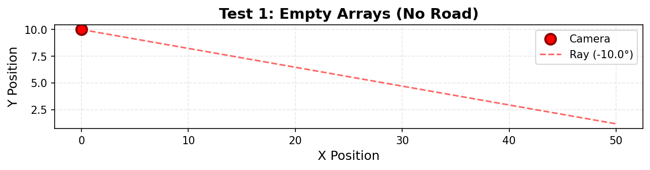
Test 1: Empty Arrays - No road to intersect
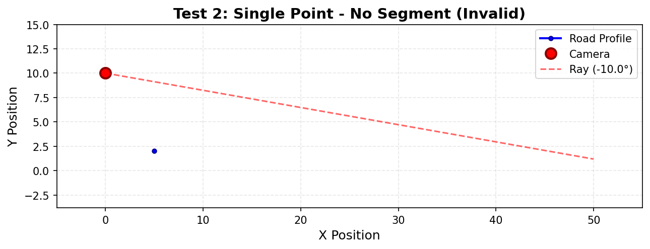
Test 2: Single Point - No segment (invalid)
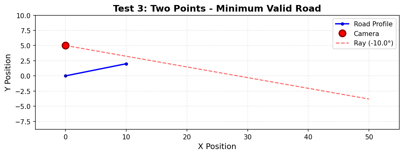
Test 3: Two Points - Minimum valid road (one segment)
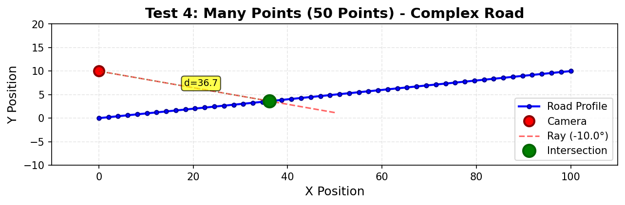
Test 4: Many Points (50 points) - Complex road
Angle Class Tests (5 tests):
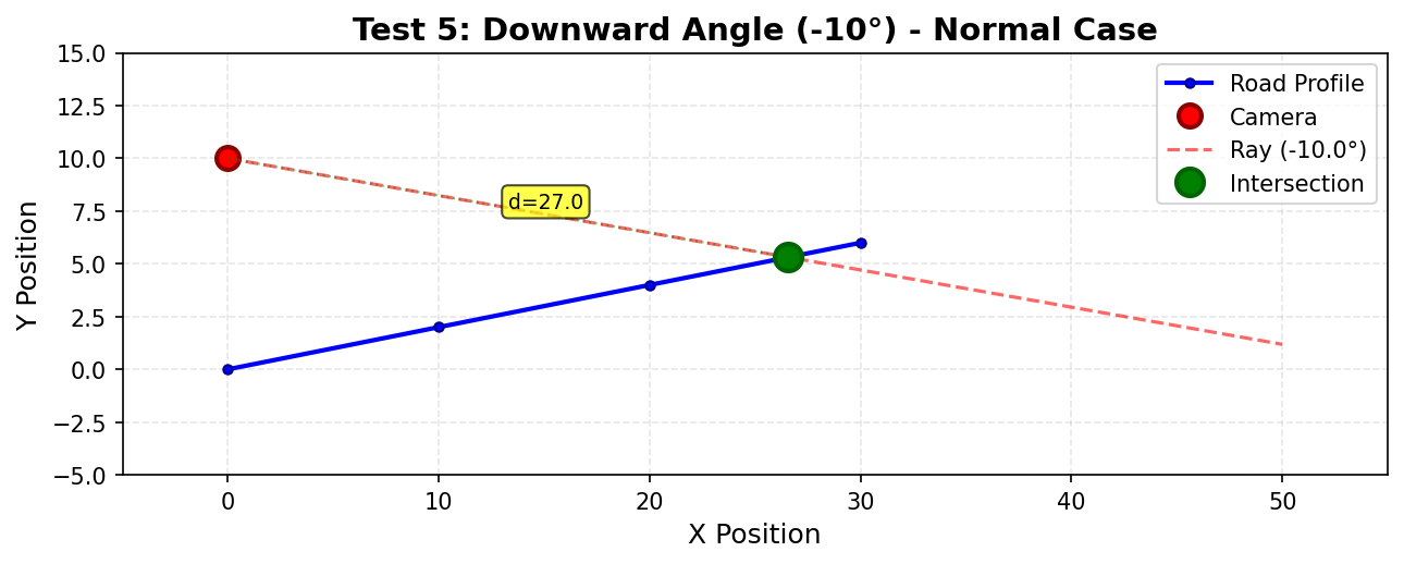
Test 5: Downward angle (-10°) - Normal case
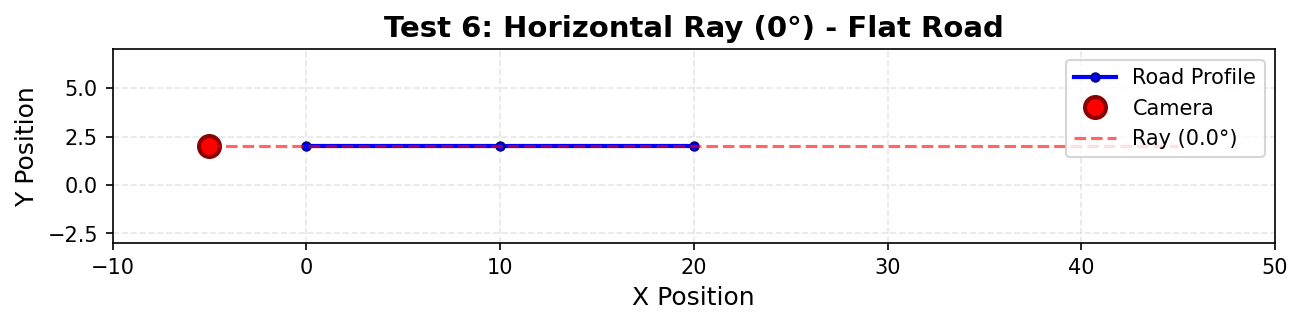
Test 6: Horizontal ray (0°) - Flat road at same level
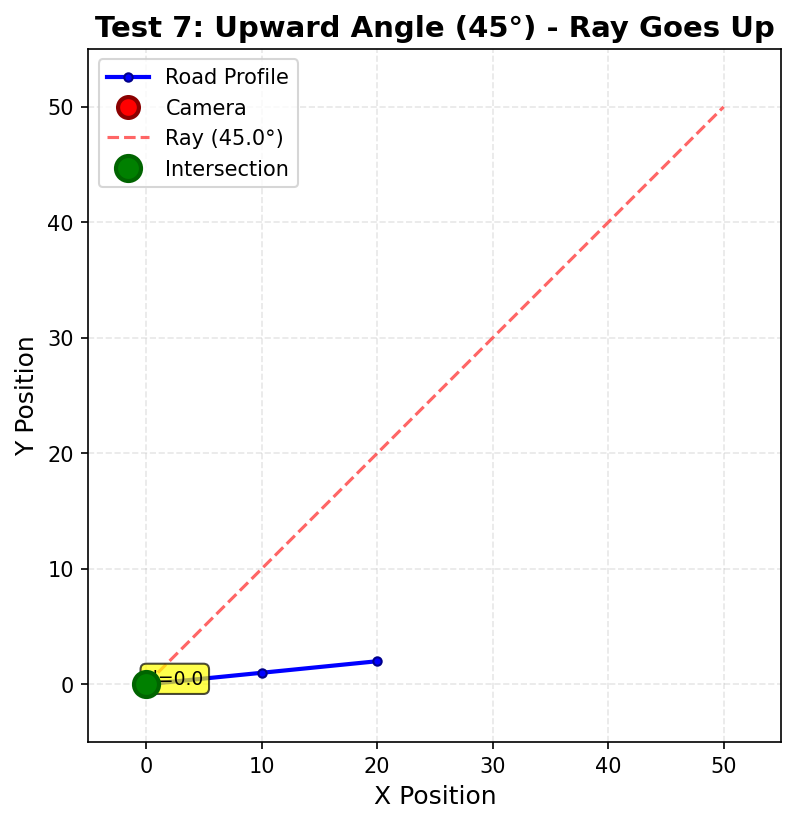
Test 7: Upward angle (45°) - Ray goes up
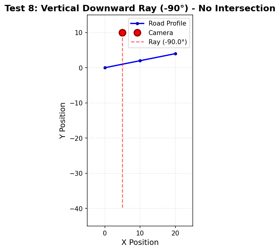
Test 8: Vertical downward (-90°) - No intersection
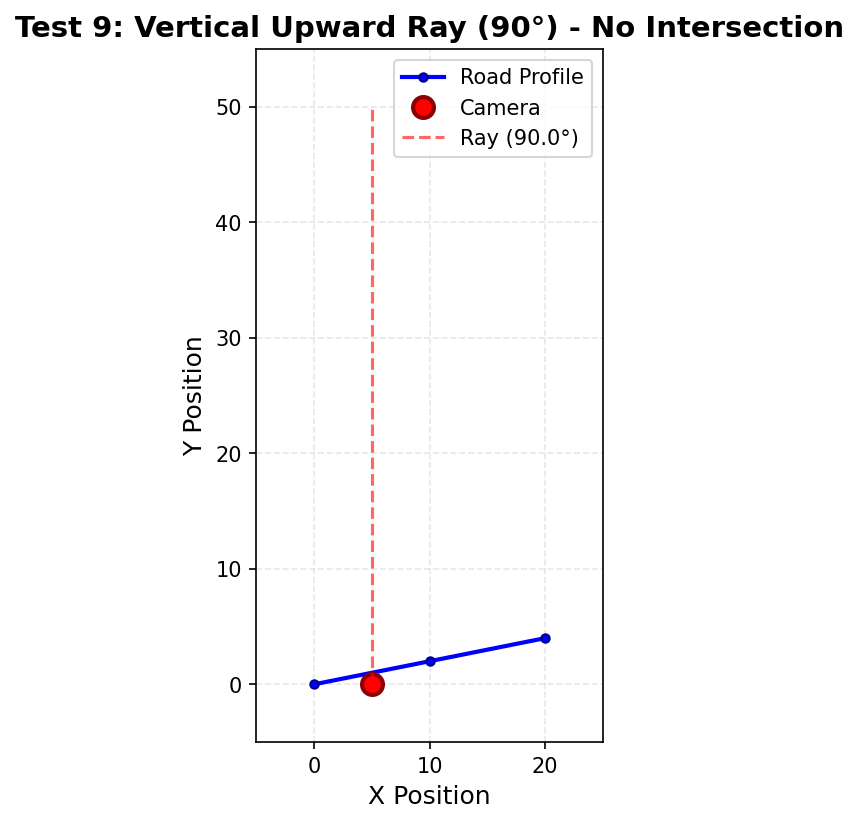
Test 9: Vertical upward (90°) - No intersection
Camera Position Tests (6 tests):
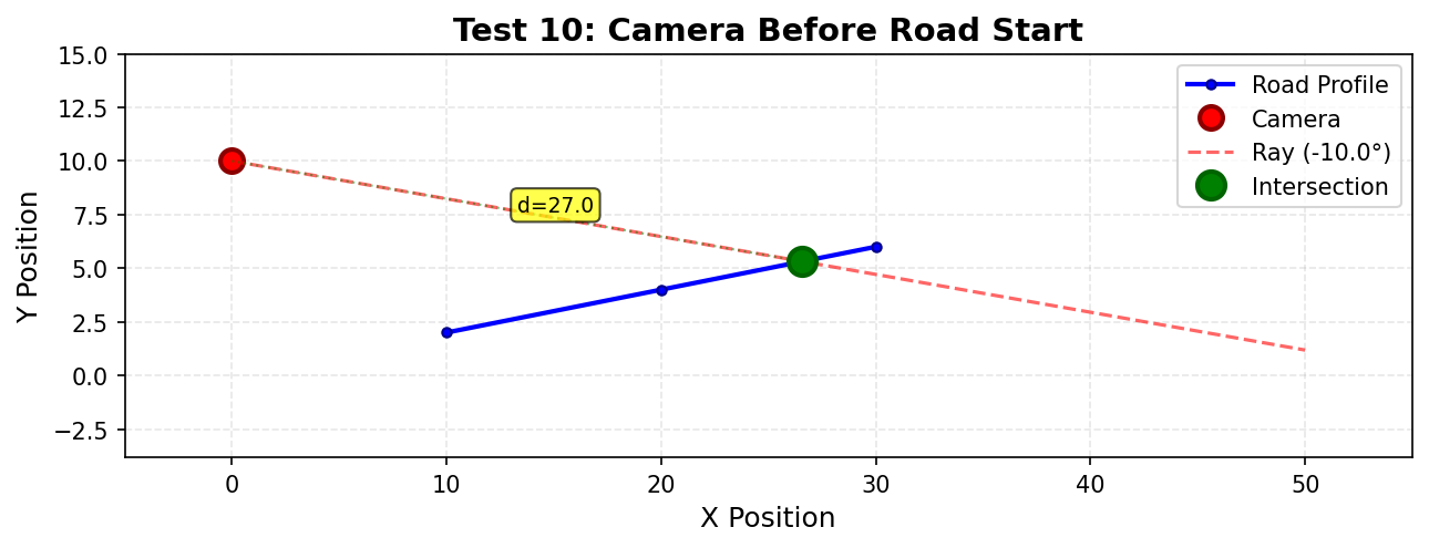
Test 10: Camera before road start - Ray travels forward
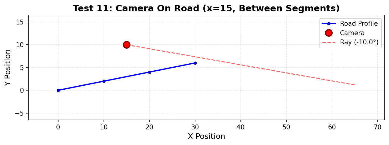
Test 11: Camera on road - Between segments
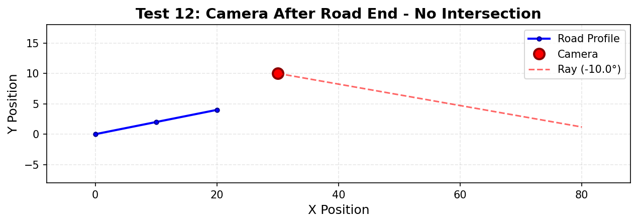
Test 12: Camera after road end - No intersection
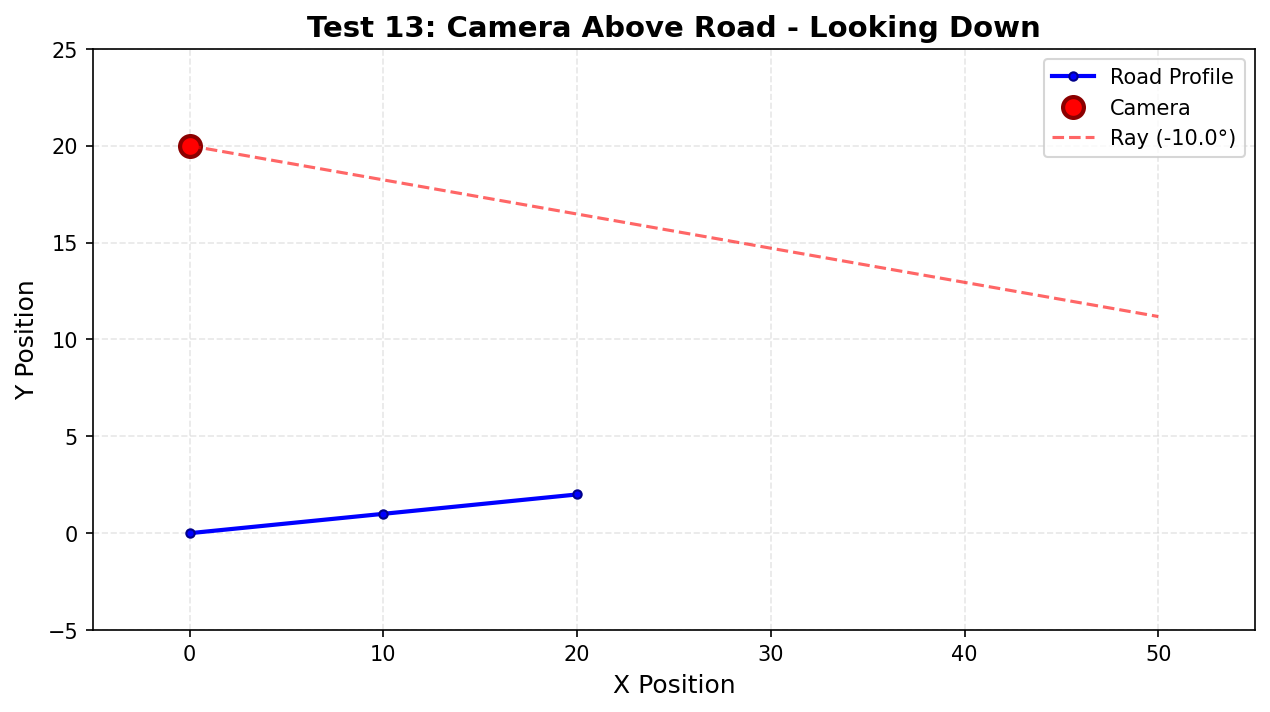
Test 13: Camera above road - Looking down
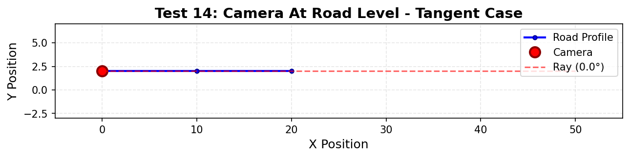
Test 14: Camera at road level - Tangent case
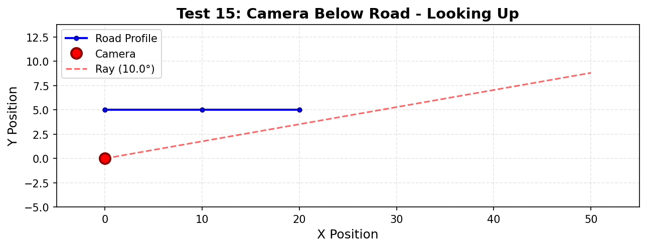
Test 15: Camera below road - Looking up
Outcome-Based Tests (4 tests):
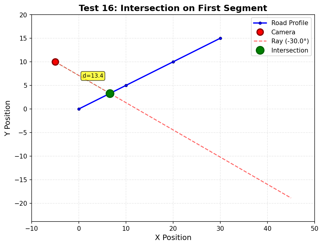
Test 16: Intersection on first segment
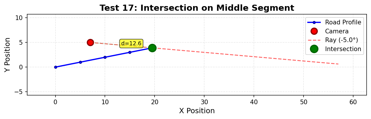
Test 17: Intersection on middle segment
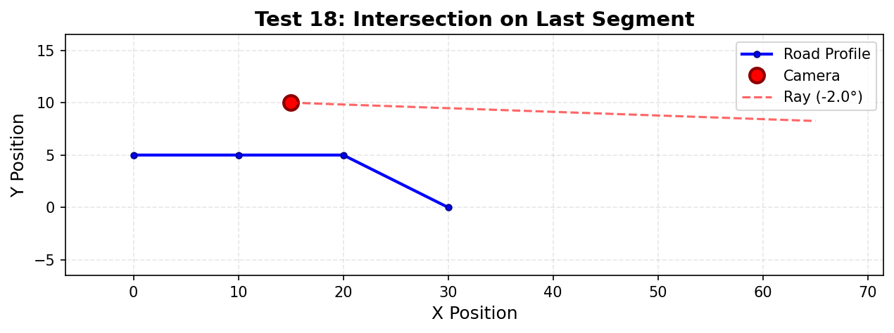
Test 18: Intersection on last segment
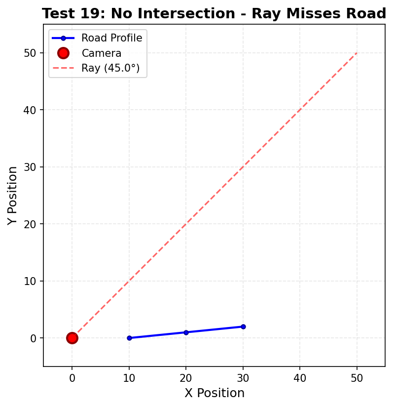
Test 19: No intersection - Ray misses road
Road Shape Tests (3 tests):
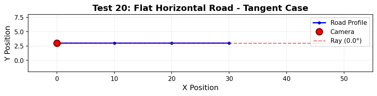
Test 20: Flat horizontal road - Tangent case
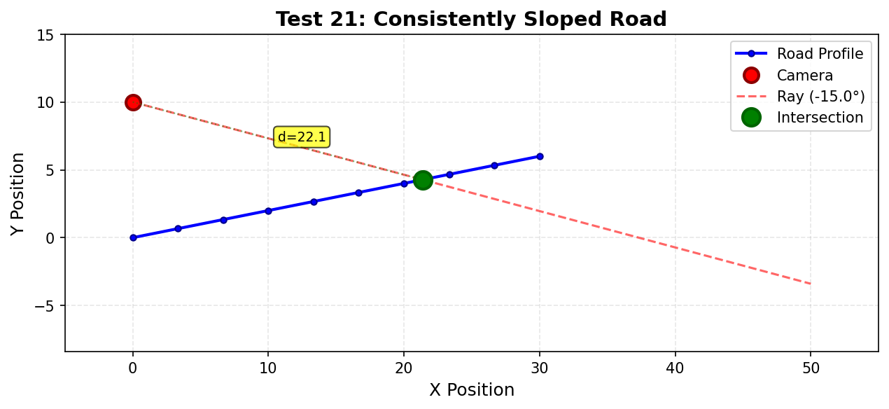
Test 21: Consistently sloped road
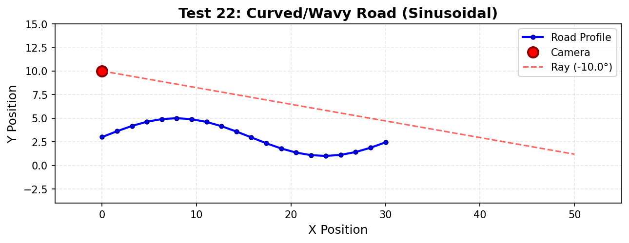
Test 22: Curved/wavy road (sinusoidal)
Why Visual Testing Matters:
These illustrations reveal insights that are hard to see from code alone:
- Geometric intuition: You can immediately see whether a test case makes physical sense
- Edge cases become obvious: Tangent rays, parallel lines, and boundary conditions are visually clear
- Missing test cases: Looking at the diagrams, you might notice scenarios you forgot (e.g., “What if the camera is inside a valley in the road?”)
- Debugging aid: When a test fails, visualizing it helps you understand whether the bug is in the test or the code
Important insight - Same output, different input dimensions:
Notice that Test 2 (Two Point Road) and Test 8 (Camera Above Road) both show NO intersection - the ray misses the road. But they’re testing completely different things!
Test 2 Math:
- Camera at (0, 5), ray at -10°
- Ray equation:
y = 5 - 0.176x - Road: (0, 0) → (10, 2), equation:
y = 0.2x - Ray and road lines would intersect at
x ≈ 13.3 - But the road ends at x=10! → No intersection
Test 8 Math:
- Camera at (0, 20), ray at -10°
- Ray equation:
y = 20 - 0.176x - Road: (0, 0) → (10, 1) → (20, 2)
- Ray would intersect at
x ≈ 72.5 - But the road ends at x=20! → No intersection
Why both tests are necessary:
- Test 2 validates: “Can the function handle a minimal road structure (just 1 segment)?”
- Test 8 validates: “Can the function handle a camera positioned far above the road?”
This demonstrates a crucial testing principle: You need to cover different input dimensions even if they produce the same output! Just because two tests both return None doesn’t mean they’re redundant - they may be exercising different equivalence classes (structural vs. positional).
Practical tip: When testing complex geometric functions, always create visualization tools early in development. They pay for themselves many times over in debugging time saved!
Key Insights from find_intersection Analysis:
- Complexity Explosion: This function has 5 parameters with:
- 5 structural classes (array lengths)
- 5 angle classes
- 6 camera position classes
- 4 outcome classes
- Potential combinations: 5 × 5 × 6 × 4 = 600 test cases!
- AI Limitations: When you ask an LLM to “write comprehensive tests for find_intersection”, it will likely:
- ✅ Generate good structural tests (empty, single, many)
- ✅ Generate angle tests (downward, horizontal, vertical)
- ❌ Miss camera position classes (below road, after road)
- ❌ Miss outcome-based classes (intersection on specific segment)
- ❌ Miss road shape classes (flat, sloped, curved)
- Human Insight Required: You need to:
- Read the code to understand logic branches
- Think about geometric edge cases (tangent, parallel)
- Consider physical constraints (camera behind road)
- Test actual behavior (does vertical angle really return None?)
Practical Approach:
You don’t need all 600 tests. Instead:
- Cover each dimension with at least 2-3 tests
- Focus on high-risk combinations (e.g., empty array + any angle)
- Use LLM for boilerplate, human for completeness
- Aim for ~20-30 tests covering key equivalence classes
This is realistic testing – comprehensive enough to catch bugs, practical enough to maintain!